How to Calculate Standard Deviation in Excel

In this video tutorial, we’re going to work through a specific example to demonstrate how to calculate the standard deviation in Excel in a quick and easy way. We’re also going to talk about the difference between the functions STDEV.S and STDEV.P and how to use both correctly in a data analysis.

What is Standard Deviation

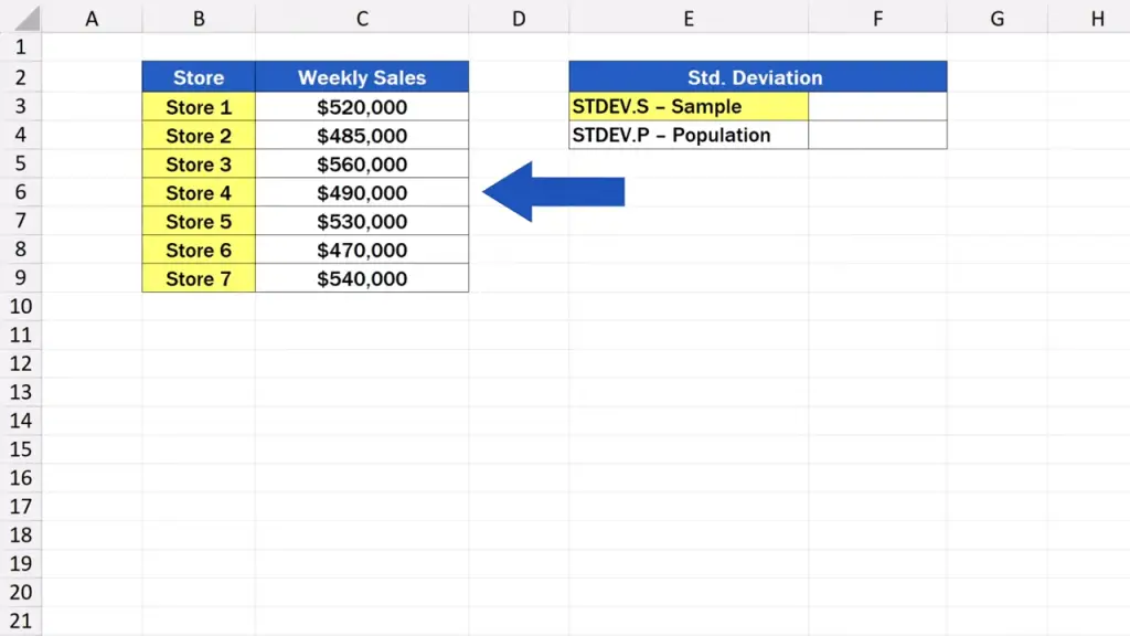
Let’s now take a look at this simple data table, which stores weekly sales in seven different shops.

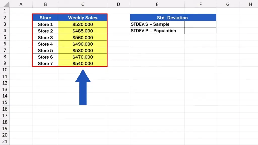
Our aim is to find out how much these figures deviate from the average. And that’s exactly what the number called standard deviation states. Standard deviation is a great way to express how spread out the sales of the individual stores are around the average.

A low number shows that all stores made roughly the same figure. But if the number is high, there are significant differences among the stores, which basically means that there are stores that sold much less or much more in comparison to other stores.

Difference Between STDEV.S and STDEV.P Explained

In Excel, there are two functions to calculate the standard deviation. One of them is marked STDEV.S, the other one STDEV.P.

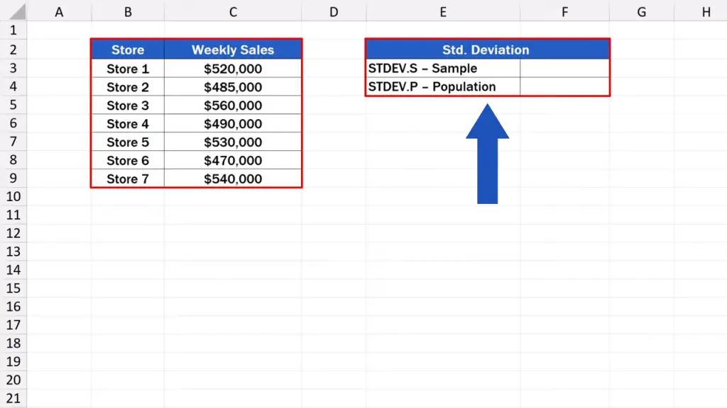
And here it comes – we’re going to take a look at what the difference between these two functions is and which one to use when.

Let’s start with the function STDEV.S. We can use this function when we work with only a sample, not the whole group of data.

For example, there are data from just seven stores out of all 100. Or we’ve got results of ten students out of the class of 30. In these cases, we use STDEV.S.

Actually, this is the function used most commonly to calculate the standard deviation. Normally, we haven’t got all the data in a group at our disposal. We’ve usually got just a sample. Excel then corrects the calculation with a little buffer added to the number expressing the standard deviation, because the result without this correction could simply be too optimistic.

On the other hand, we use the function STDEV.P If we’ve got a complete data set available.

This means working with the whole data population, for instance, when we work with all 100 stores or when we take into account the results of all 30 students in the class. In those cases, Excel doesn’t correct the calculation and goes ahead with the exact number it calculated for the whole population.

Now, let’s have a look at it in practice.

How to Calculate STDEV.S in Excel

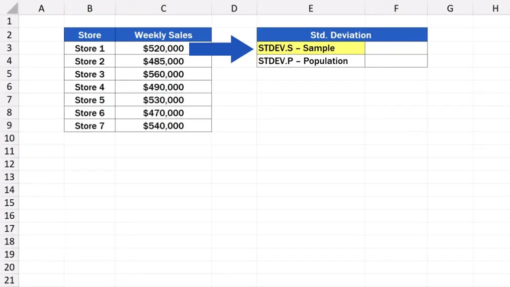
First, we click on the target cell, the cell where we want the result to appear. We start with the STDEV.S calculation.

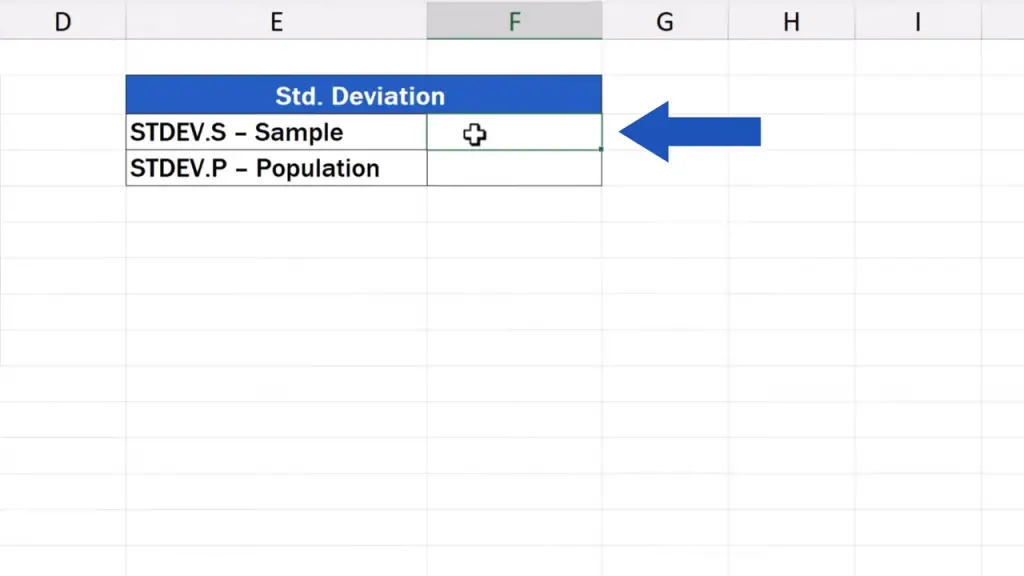
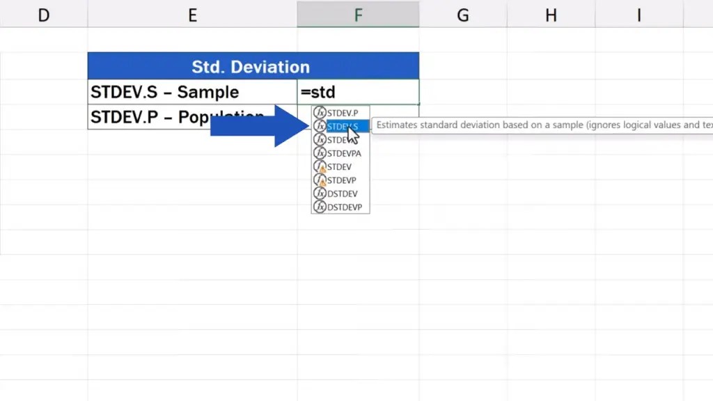
So, we click on F3, start typing the equal sign and select the function ending in ‘S’. We click on the function.

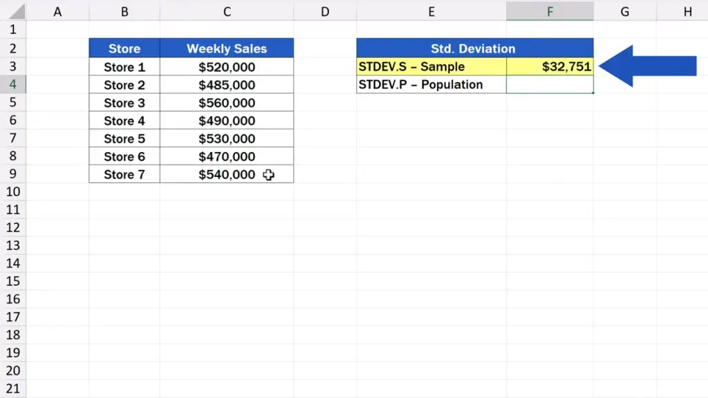
And now it’s time to identify the cells range containing the data we want to include in the calculation. We select the weekly sales for all seven stores, press Enter and here we go!

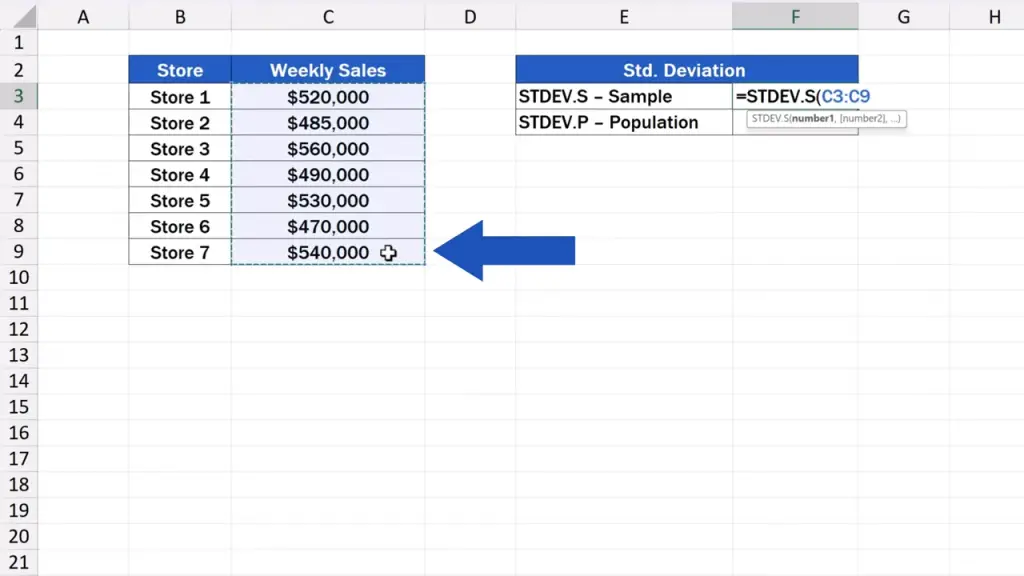
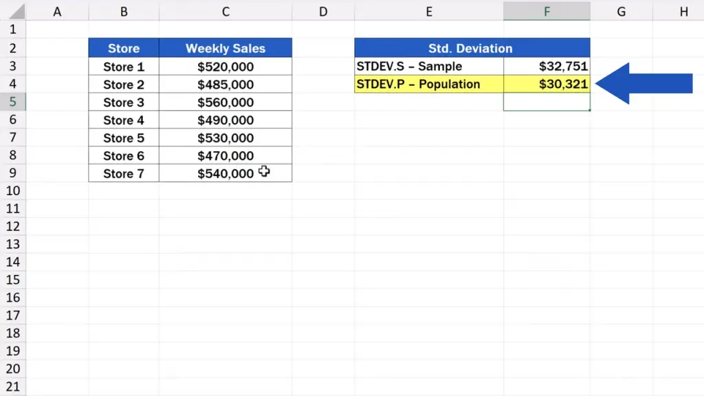
Excel has calculated the standard deviation for a sample, the result coming up to 32 751 US dollars.

How to Calculate STDEV.P in Excel

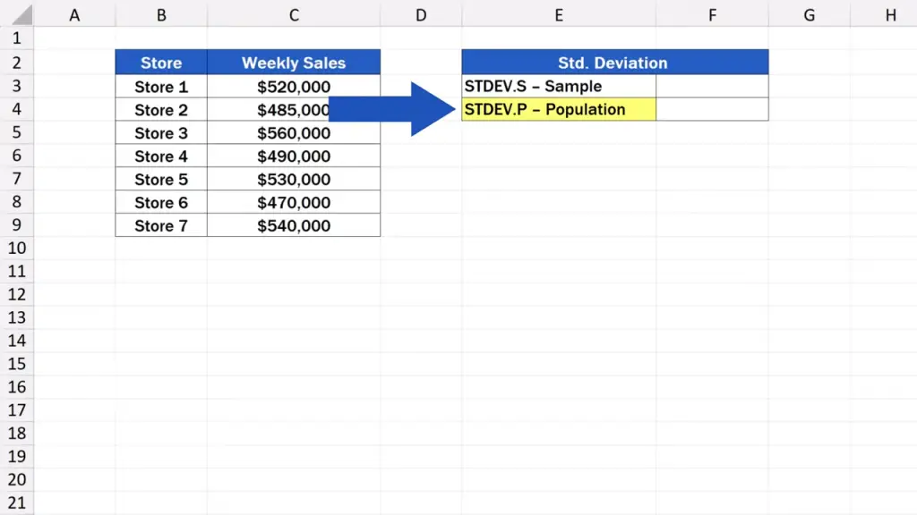
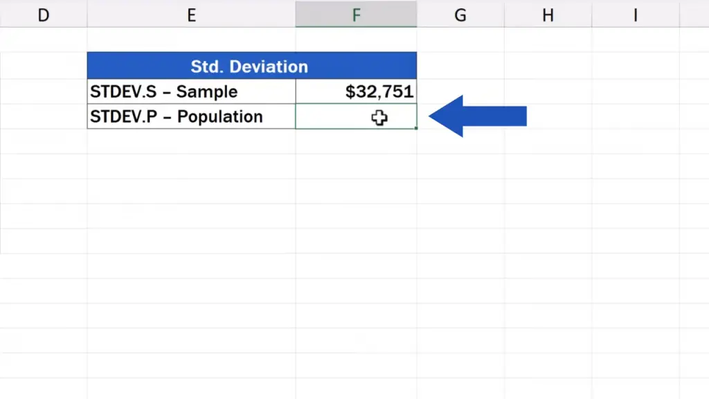
The same way we can calculate the standard deviation for a population. We click on the cell F4.

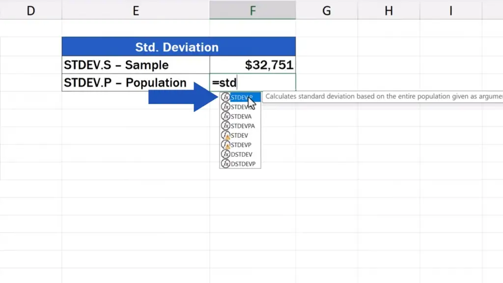
We start typing the function name, but now we choose the one ending in ‘P’.

Then we specify the relevant cells range, again, we press Enter and that’s it!

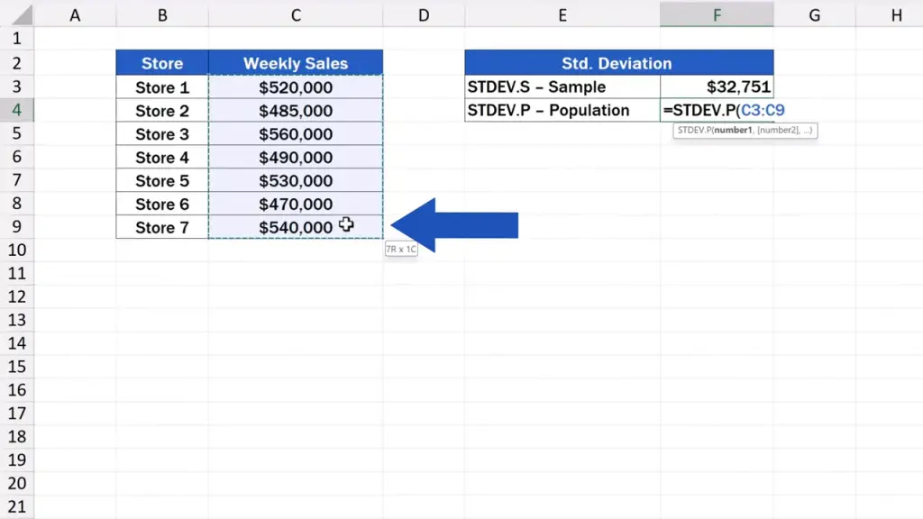
The standard deviation for the population is 30 321 US dollars.

These numbers tell us how much the sales of individual stores differ from the average sales value. Here, the average sales value is approximately 514 000 US dollars.

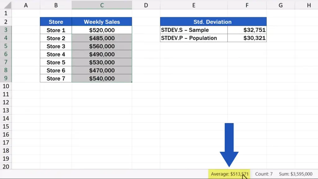
Also, the rounded standard deviation number is 33 000 dollars, so it tells us that most of the stores make sales within the range of plus or minus 33 000 dollars from the average sum.

The difference between the STDEV.S and STDEV.P calculation, which is the difference between 32 751 and 30 321 dollars means that if we take into account just a sample of stores, Excel counts on results possibly differing in the rest of the stores in the population. That’s why Excel states a slightly higher value of the standard deviation – to give us a more realistic picture about variance.

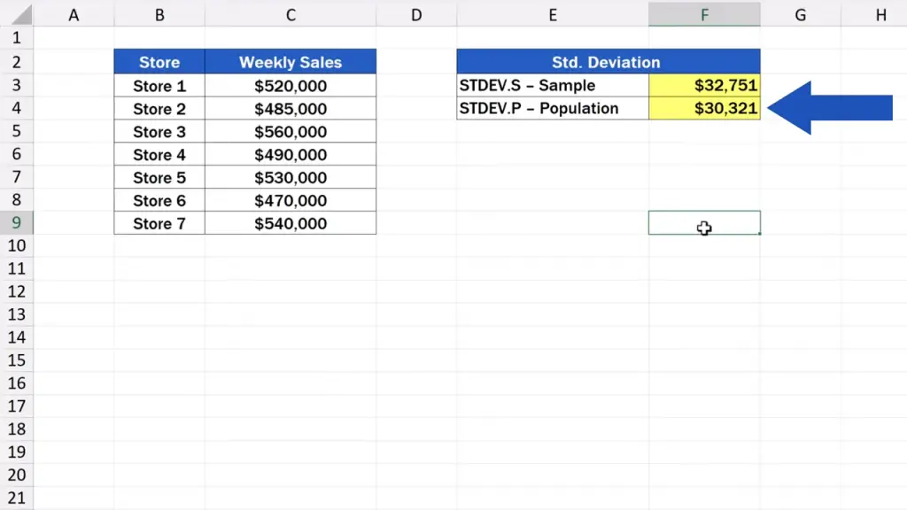
However, if we work with the whole population, we’ve got all the necessary data at hand, so there’s no need for a buffer, which means the number stated as the result is exactly the same as came out of the calculation.

So, those have been two ways to calculate the standard deviation, which you can now use with the data you’re working with.

And before we wrap it up, here’s a question for you: which of the functions will you most probably use when calculating the standard deviation the next time? Will you be working with a sample or the whole population? Share your opinion in the comments section below. We’ll be happy to hear from you!

Don’t miss out a great opportunity to learn:

• How to Count Unique Values in Excel
• How to Calculate a Rank in Excel
• How to Calculate the Median in Excel

If you found this tutorial helpful, give us a like and watch other tutorials by EasyClick Academy. Learn how to use Excel in a quick and easy way!

Is this your first time on EasyClick? We’ll be more than happy to welcome you in our online community. Hit that Subscribe button and join the EasyClickers!

Thanks for watching and I’ll see you in the next tutorial!