How to Change the Currency in Excel
Today we’re going to go through a quick and easy guide on how to change the currency in Excel. These simple steps will make sure that the financial figures in a data table show in the right format – just as you need!
Ready to start? So, let’s get into it!
How to Select Cells for Currency Formatting
To set a specific currency for certain figures in a data table we start with selecting all the cells where we want to change the currency. We can click on just one cell or select multiple cells at the same time, depending on what we need.
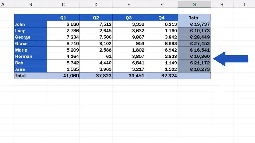
Here we’ll be working with the column ‘Total’, so we select the whole column and move on to the next step.
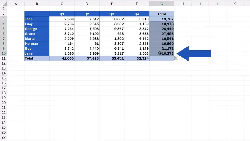
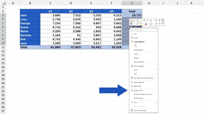
Now, we use a right-click to get to this list of options where we look up ‘Format Cells’ and click on it.
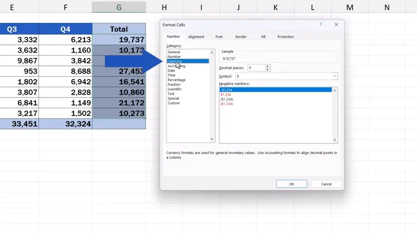
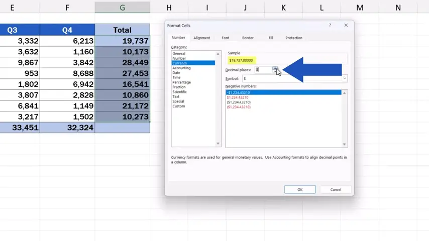
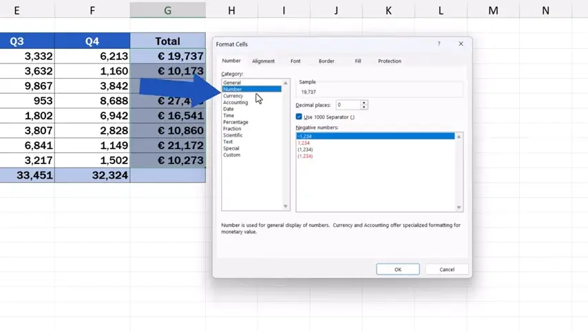
We’ll see a pop-up window, which we’ll move up here a little bit, and in the field ‘Category:’ we’ll search for ‘Currency’ and again, click on it.
How to Choose a Specific Currency in Excel
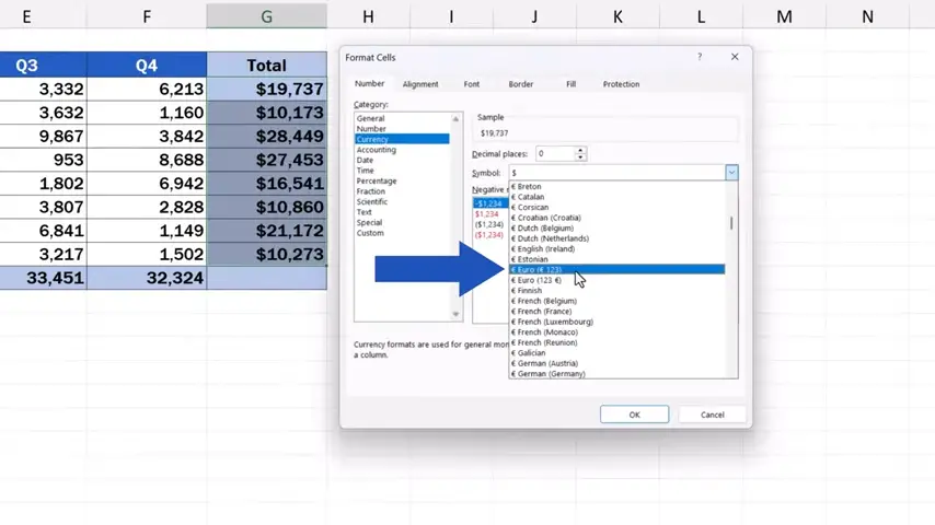
On the right, we can select the currency symbol we need. There’s a really huge list of currencies from all over the world available in the drop-down list. We can even find Bitcoin among them.
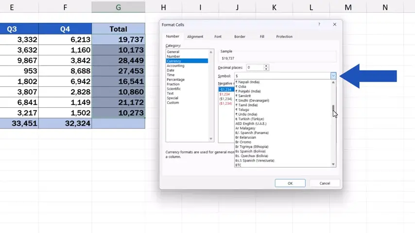
Let’s select the US dollar now and let’s have a look at more advanced settings.
For example, we can additionally set the number of decimal places to be displayed for these figures.
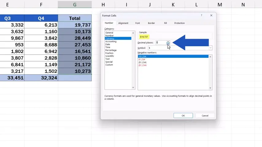
In this case, we set the number of decimal places to zero, so we actually don’t want to show any decimal places here in our figures.
Now we just press OK and that’s it!
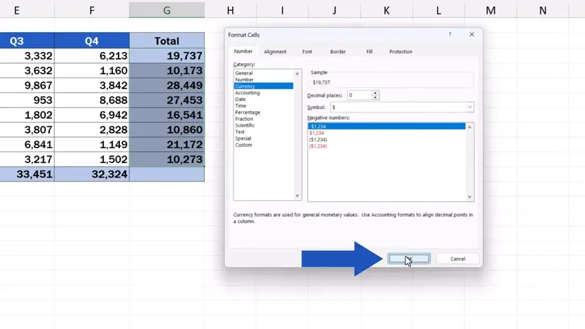
All figures in ‘Total’ show in US dollars with no decimal places.

The same way we can change the currency from the US dollar to a different one.
Simply, we select all the cells where we want to change the currency and through a right-click we choose the option ‘Format Cells’ again.

In the drop-down list we look up the currency we need. Let’s change the currency to Euro now.
Press OK and here we go! The format’s been updated again and the totals show in Euros, just as we’ve selected.
How to Remove the Currency Symbol in Excel
And it’s very simple to display no currency next to the figures, too.
We select the target cells again, do a right-click and select ‘Format Cells’ one more time.
But watch out here!
If you’d like to show no currency next to the figures, in the field ‘Category’ click on the option ‘Number’.
Of course, we can set the number of decimal places to be displayed here, too. Or we can tick or untick the use of the thousand separator, whatever works better for us.
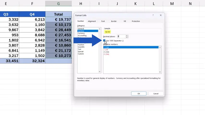
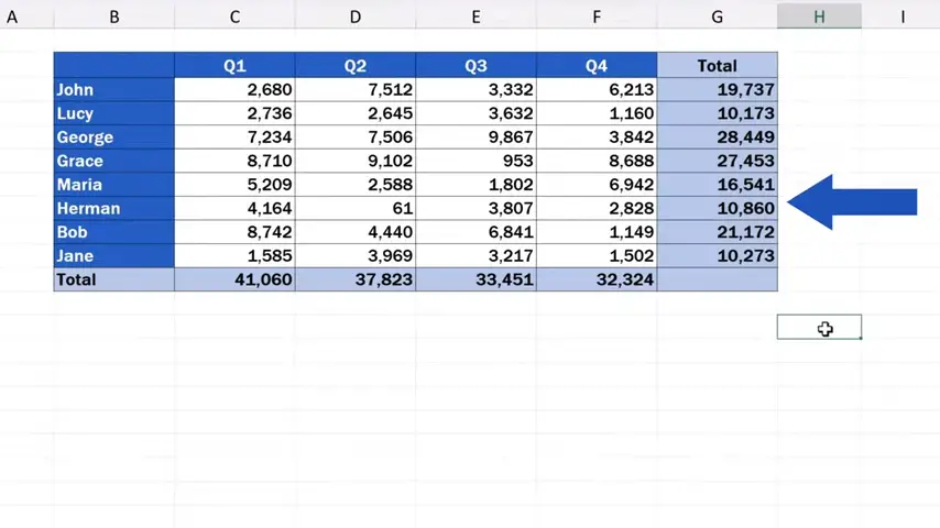
We’ll keep the number of decimal places at zero, we’ll use the separator, and we’ll finally press OK and there it is!
The figures show as numbers with no currency symbol whatsoever.
Don’t miss out a great opportunity to learn:
If you found this tutorial helpful, give us a like and watch other tutorials by EasyClick Academy. Learn how to use Excel in a quick and easy way!
Is this your first time on EasyClick? We’ll be more than happy to welcome you in our online community. Hit that Subscribe button and join the EasyClickers!
Thanks for watching and I’ll see you in the next tutorial!

 How to Subtract a Percentage in Excel
Welcome! Today we’re going to talk about the simplest way how to…


