How to Freeze Rows in Excel

In this short tutorial, you’ll see a simple way how to freeze cells in Excel. You can freeze rows to always see the header of your table when scrolling down the spreadsheet, and we’ll also have a look at how to freeze columns in case you want to lock the first column in its position while you’ll be scrolling across the data in the table.

Here we go!

See the video tutorial and transcription below:

See this video on YouTube:
https://www.youtube.com/watch?v=yw_WsTSh9RE

Freezing rows and columns in Excel is an amazingly handy thing. Especially with tables containing lots and lots of data. Here is an example!

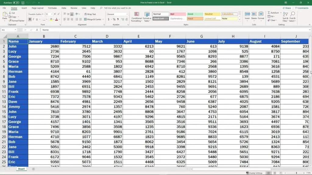
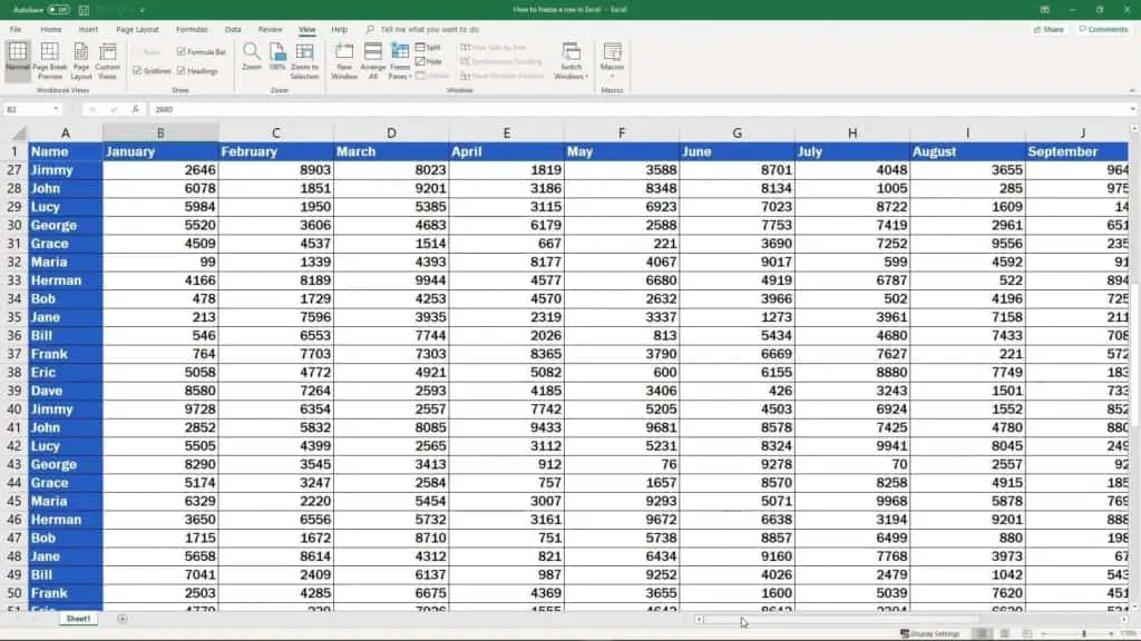
Let’s say you work in a spreadsheet such as this one. If you keep scrolling down, you might notice that the header – in this case the months – disappears.

Also, if you scroll across to the right, columns to the left might get out of sight, too. For example, now we cannot see the names of employees anymore.

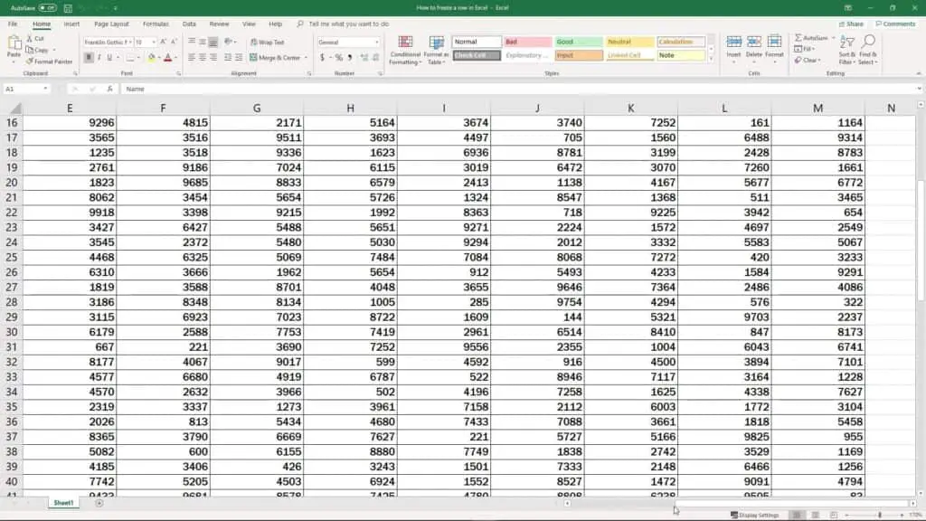
This way, it might get very hard not to get lost in data. That’s why we’ve got the function ‘freeze rows/columns’ – to get a clear overview of the information in the table.

Let’s scroll back now and see how we can freeze cells.

First thing, we’ll click on a cell which marks the rows and columns we want to freeze. It’s the first row and the first column here in our table, and that’s why we click on the cell B2.

The marking works in the way that all rows above as well as all columns to the left of the marked cell will freeze.

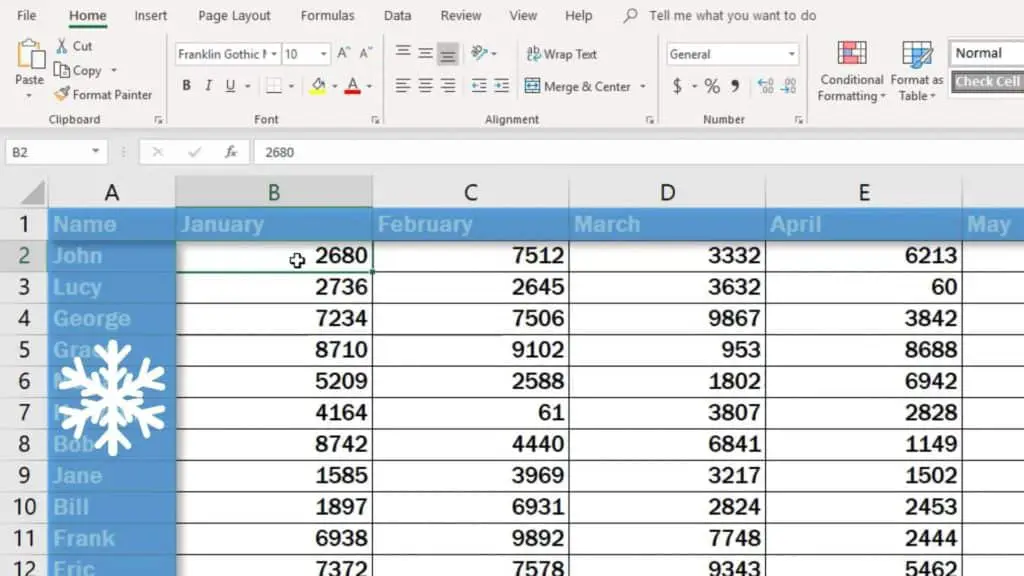
The header along with the column with employees’ names will get ‘locked’ in their position on the screen, so you’ll see them all the time, no matter how far into the spreadsheet you scroll.

How to Freeze Only the Top Row in Excel

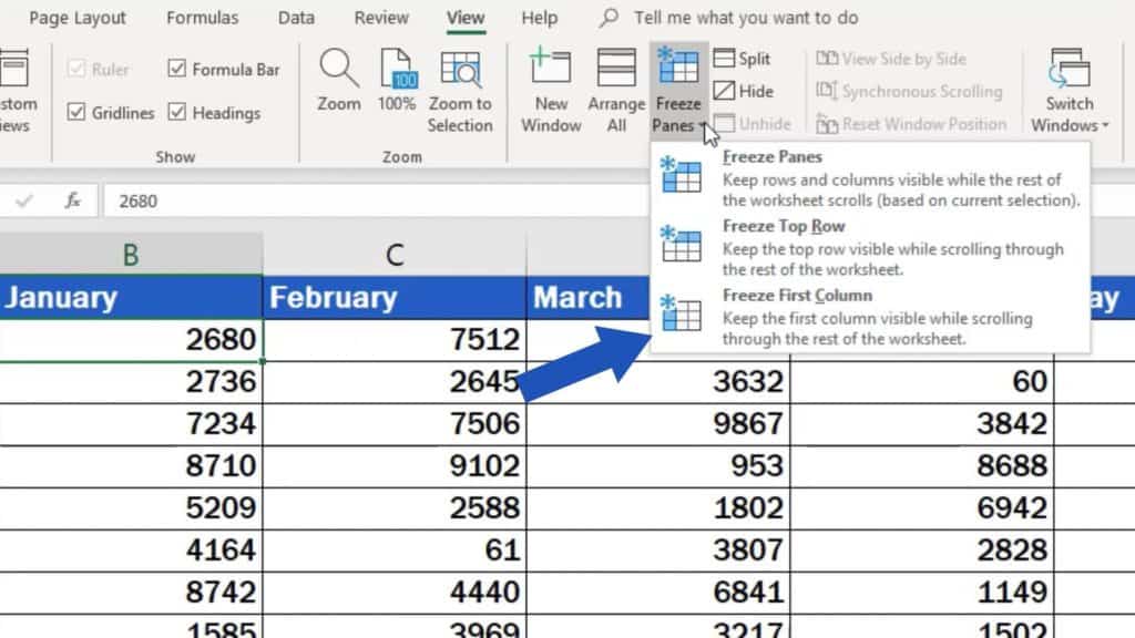
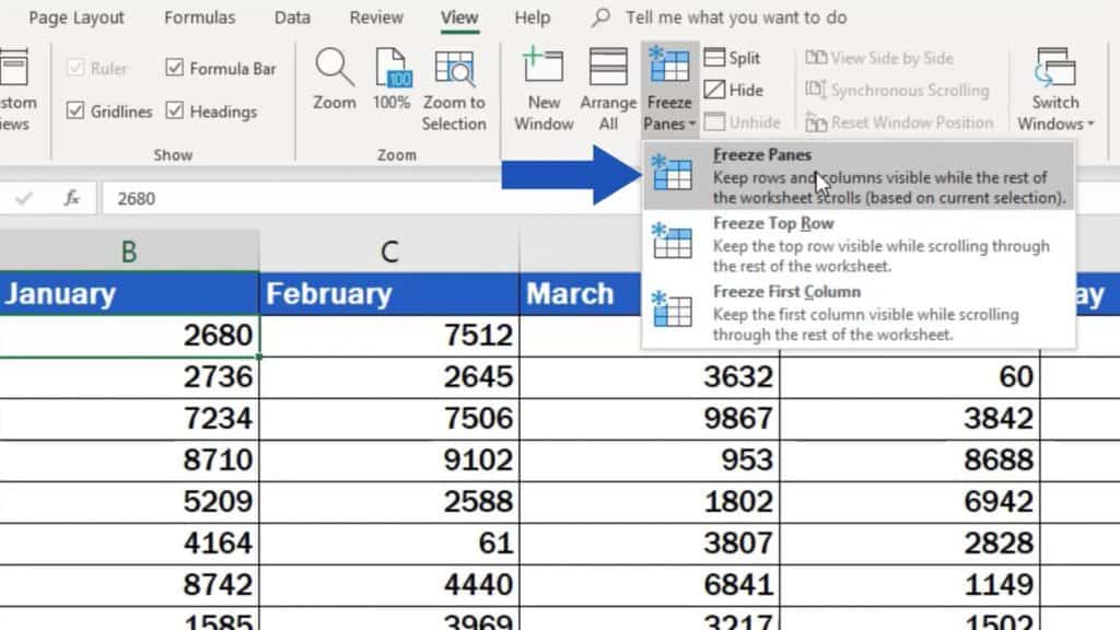
Once you’ve marked the selected cell, click on the tab ‘View’, then go the section ‘Window’ and select ‘Freeze Panes’. If you want to freeze only the top row or just the left-hand column, go for one of the other options – ‘Freeze Top Row’ or ‘Freeze First Column’.

How to Freeze Only the Left-Hand Column in Excel

But what we want now is to freeze the rows and columns just like we said before. So, we’ll go for the first option – ‘Freeze Panes’.

Good job!

The header with months and the column with names are visible all the time now! The data in these cells are still on the screen even though I scroll a bit further down or to the right in the spreadsheet, which makes it much easier to read through and process the data.

How to Unfreeze panes in Excel

To undo the formatting, go back to the ‘View’ tab, and in the section ‘Window’ select the option ‘Unfreeze Panes’.

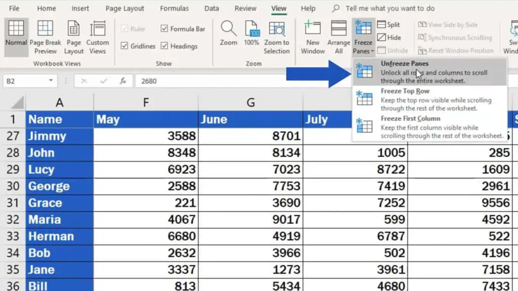
This will remove the formatting change and ‘unlock’ the row and column so that they disappear when you scroll down or across to the right.

Are you wondering:

• How to Lock Cells in Excel
• How to Insert Row in Excel
• How to Protect Excel Sheet with Password
• How to Merge Cells in Excel

If you’ve found this tutorial helpful, like us and subscribe to receive more videos from EasyClick Academy. Look at more tutorials that help you use Excel quick and easy!

See you in the next tutorial!