How to Hide Rows in Excel

In this short tutorial, we’re gonna have a look at how to hide rows in an Excel spreadsheet – simple and easy! Thanks to this, you’ll be able to hide information you don’t want to share in the table.

Let’s get started!

See the video tutorial and transcription below:

See this video on YouTube:
https://www.youtube.com/watch?v=TRwWLz_-4c4

There are more ways to hide a row or rows in a spreadsheet. Here, I’ll introduce two of them.

Let’s crack on with the first one!

The first way how to hide rows in Excel

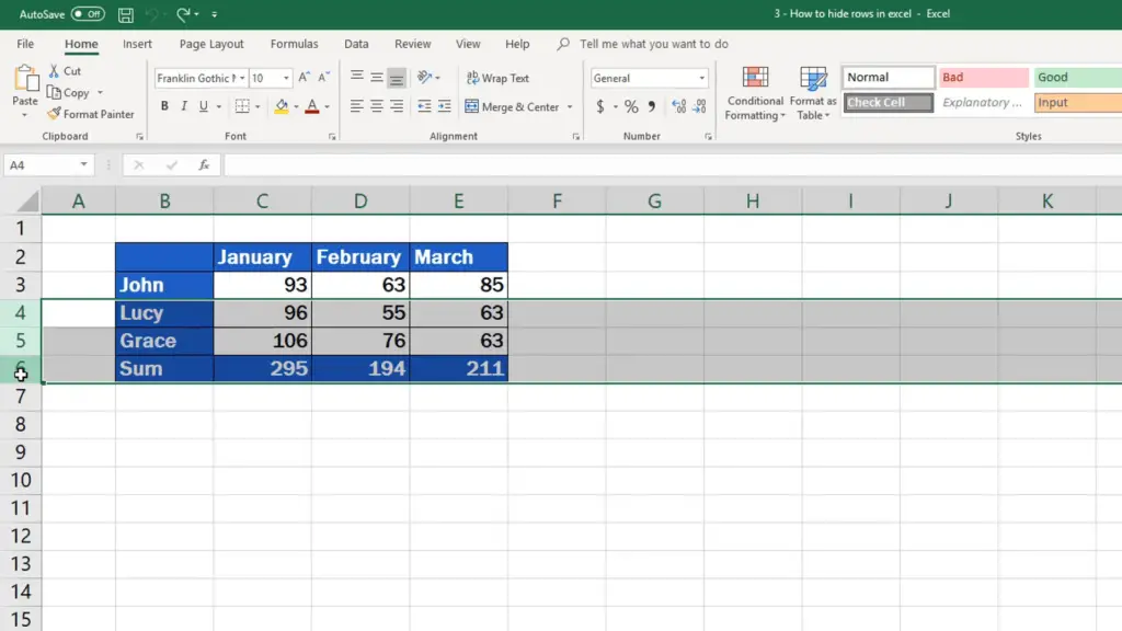
First, highlight the row you’d like to hide. This can be done through a click on the bar of numbers, selecting the relevant row. If you wish to hide more rows at once, press the Shift key and click on each of the rows you want to hide. If the rows you want to hide are not consecutive, which means they do not lie next to each other, use the Ctrl key instead of Shift.

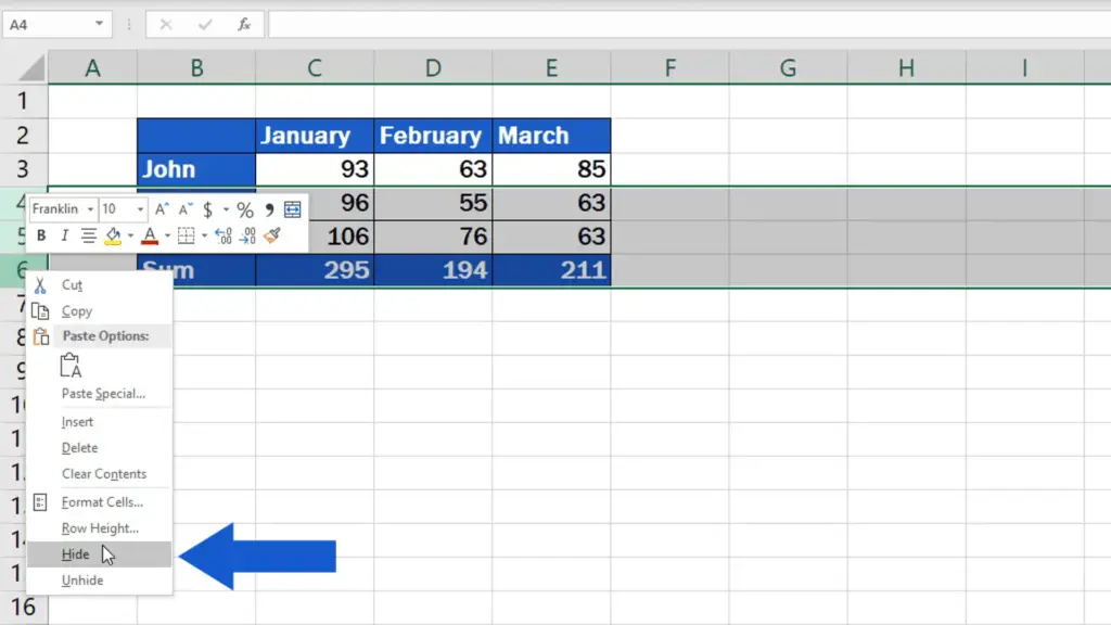
Once you’ve selected all the necessary rows, use the right-click button to see the Hide option. The hidden rows are not visible in the table on the screen. They also won’t be printed out if you were to do so with the spreadsheet. But they’ve not been deleted! You can ‘unhide’ them anytime.

The second way how to hide rows in Excel

Alright! Let’s undo the changes now and let’s have a look at the other way to hide rows, too.

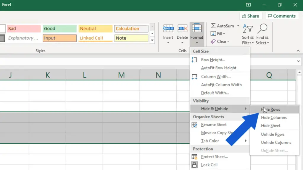
Select the rows again, this time by dragging, then go to Home tab, Cells section (or group), use Format button to get to the Format menu. Find Hide & Unhide option and select Hide Rows.

And the work’s done!

Would you like to know:

• How to Unhide Rows in Excel
• How to Hide Columns in Excel
• How to Unhide Columns in Excel
• How to Hide Sheets in Excel

If you’ve found this tutorial helpful, like us and subscribe to receive more videos from EasyClick Academy. Watch more videos that help you use Excel quick and easy!

See you in the next tutorial!