How to Highlight Blank Cells in Excel (Conditional Formatting)

In this tutorial, you’ll see how to highlight blank cells in Excel. Thanks to this function, you’ll be able to mark clearly all cells containing no data in a table of any size.

Let’s start!

See the video tutorial and transcription below:

See this video on YouTube:
https://www.youtube.com/watch?v=IBDG43yqfjA

At the beginning of this video, I’m gonna do the usual and tell you that there’s more than one way to highlight blank cells in an Excel spreadsheet.

This tutorial provides a detailed description on what to do to highlight blank cells using conditional formatting. Conditional formatting will ensure that highlighting will be dynamic, which means it will follow any change made in the table.

In other words, if there’s a blank cell in the table you’re working with, it’ll get highlighted. But as soon as you enter a value in this cell, the highlighting will disappear automatically. This method provides a great overview of which cells in a table are blank and which contain some data.

Ready to begin?

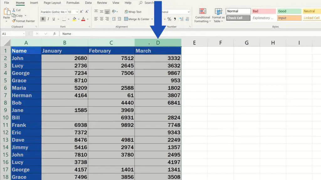
First thing that needs to be done is to mark the area in which we want to have blank cells detected and highlighted. If you’re working with a table that contains a lot of information, just select whole columns. Like this.

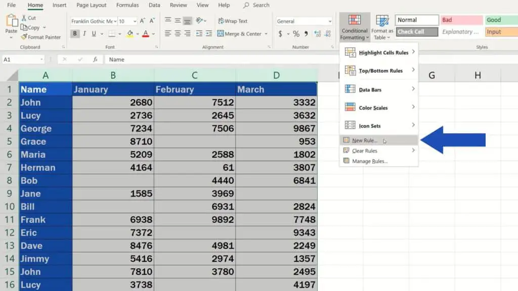
Go to group ‘Styles’, click on ‘Conditional Formatting’ and select ‘New Rule’.

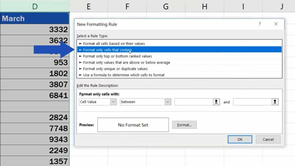
In the pop-up window, select the option ‘Format only cells that contain’.

Specify How Excel Should Format the Blank Cells

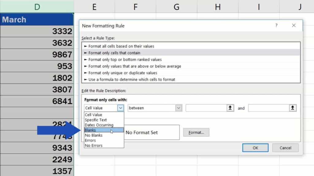
Now we’re gonna set up the rule.

We want to highlight only blank cells, so we’ll go for the option ‘Blanks’ here.

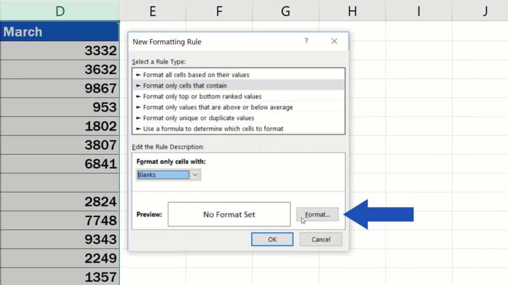
And the next step is to specify how Excel should format the blank cells within the table. Click on the button ‘Format’.

Here you’ll find various possibilities of how you can format the blank cells. We’ll now define that the blank cells will be highlighted in, let’s say, this red.

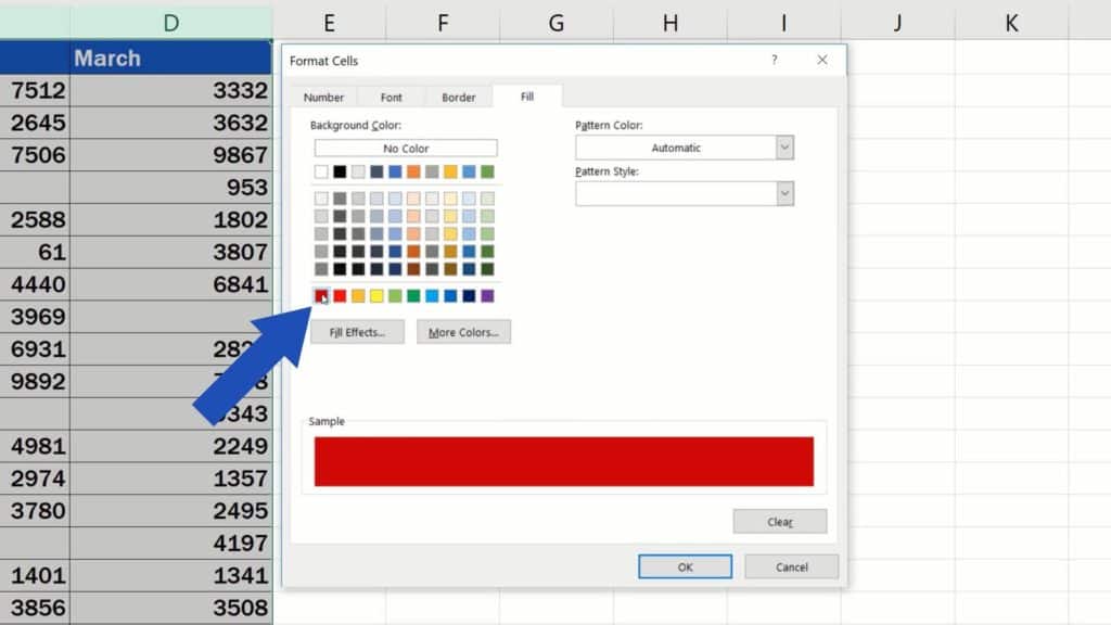
So, click on the chosen colour and confirm with OK.

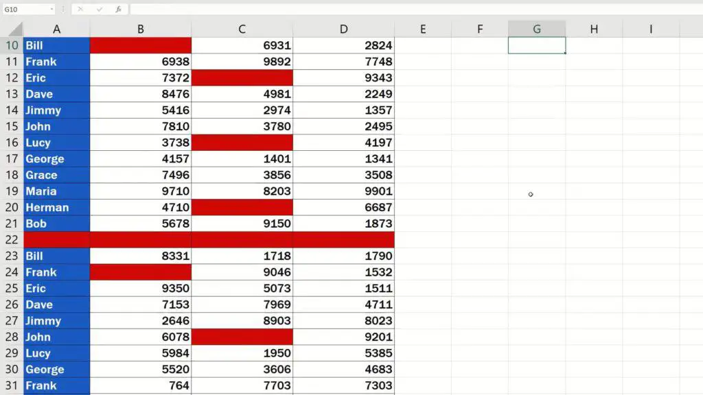
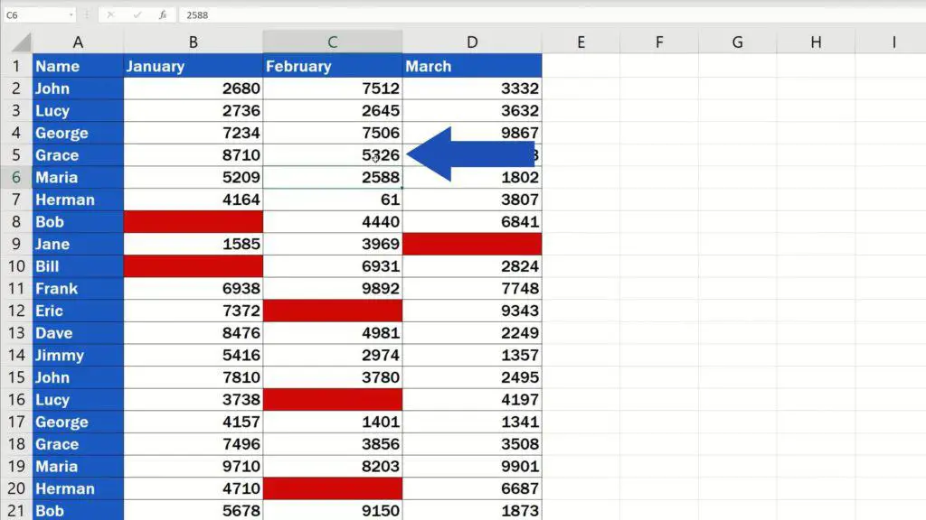
The blank cells in the table have been highlighted in red just as we wanted. And what’s even better, as you already know, the highlighting will be dynamic.

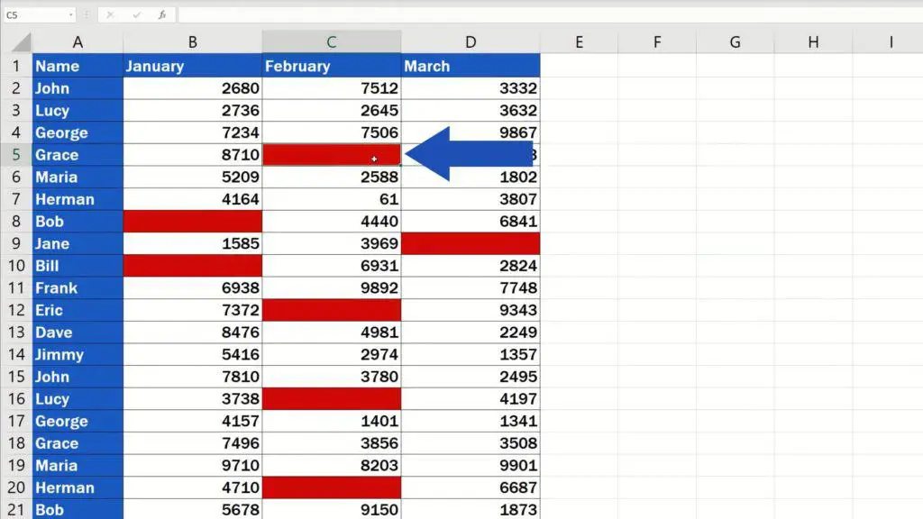
If we type some data in the cell C5, the red highlighting will disappear.

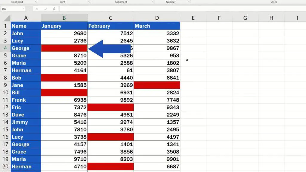
Also, if we delete the value in, for example, the cell B4, Excel will automatically highlight the cell in the colour we’ve chosen.

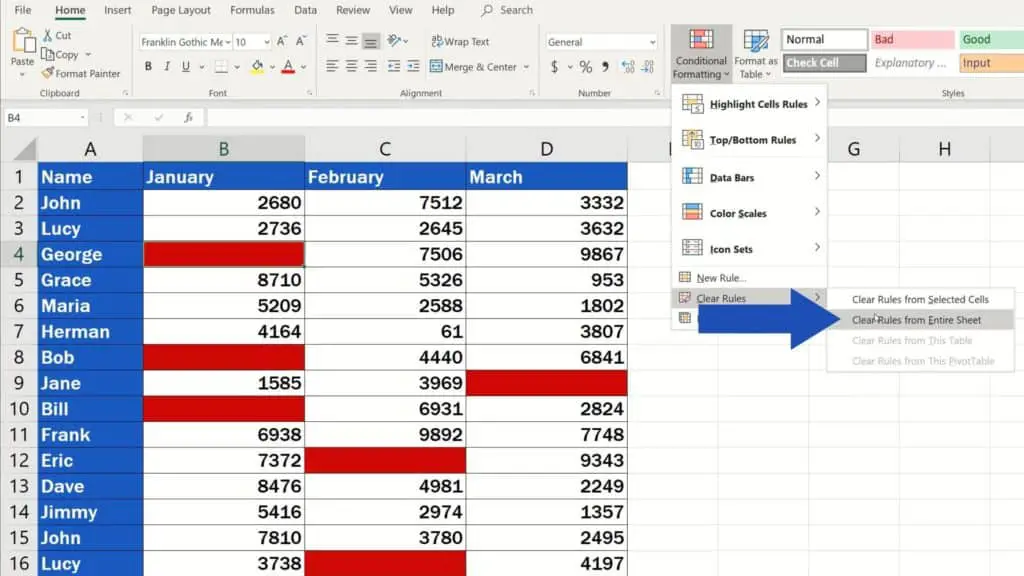
How to Turn the Function Off

And if you’d like to turn the function off, simply click on ‘Conditional Formatting’ and then ‘Clear Rules’. This can apply to a selected area or the whole spreadsheet. Select ‘Clear Rules from Entire Sheet’, and Bob’s your uncle – all the highlighting is gone!

If you’re interested in learning more about a simple way of conditional formatting, watch our upcoming videos by EasyClick Academy team.

If you found this tutorial helpful, give us a like and watch other video tutorials by EasyClick Academy. Learn how to use Excel in a quick and easy way!

Is this your first time on EasyClick? We’ll be more than happy to welcome you in our online community. Hit that Subscribe button and join the EasyClickers!

Thanks for watching and I’ll see you in the next tutorial!