How to Insert Image in Excel Cell (Correctly)

In this tutorial, you’ll learn how to insert an image in an Excel cell, in the right way. Each image inserted in the Excel sheet will be placed nice and neat within its target cell. In addition, we’ll learn to set the right formatting, so that the image could move and change size along with the cell. This comes quite handy when you need to hide or filter rows or you’re planning some further operations with the row or cell that contains the inserted the image.

Sounds like there’s a lot ahead of us, so let’s start!

See the video tutorial and transcription below:

See this video on YouTube:
https://www.youtube.com/watch?v=_lv7r8JVxW8

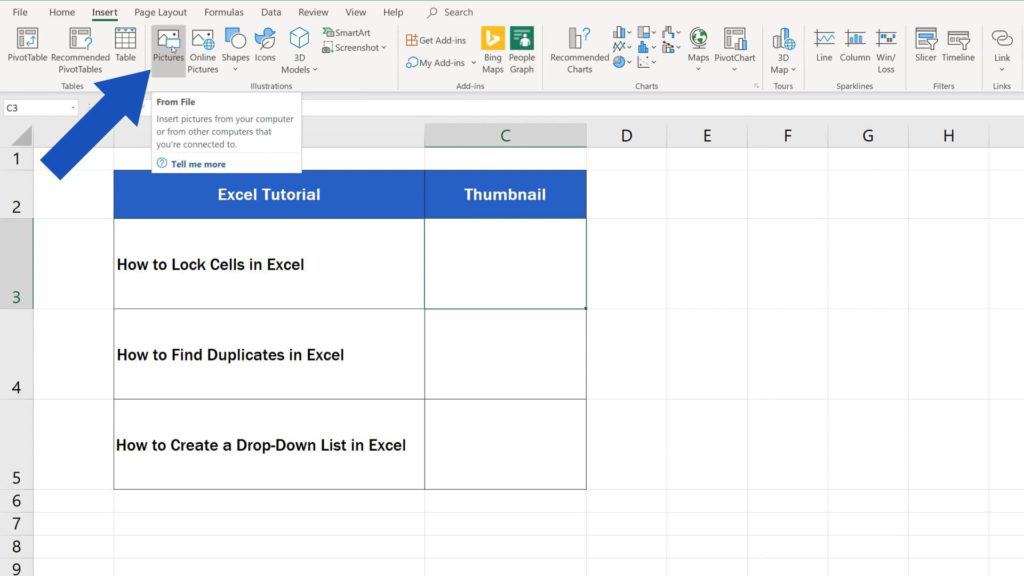
To insert an image into a spreadsheet, go to the tab ‘Insert’, then, in the section ‘Illustrations’, select ‘Pictures’.

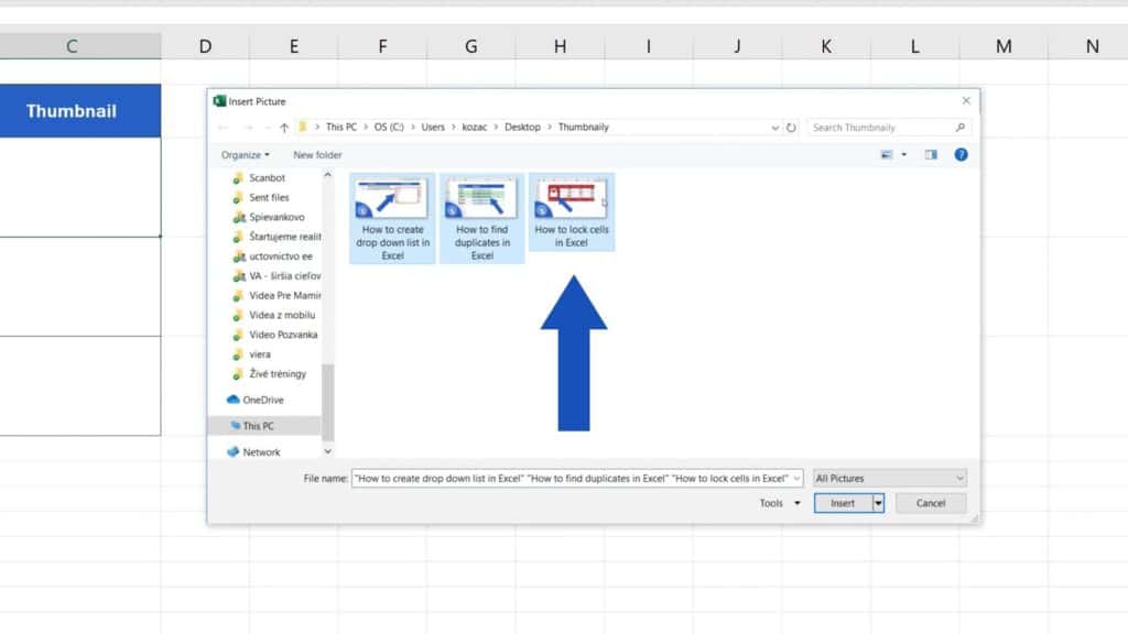
This pop-up window appears where you can browse and select pictures from your computer. You can choose one or more pictures at once and insert them into the spreadsheet area through the ‘Insert’ button.

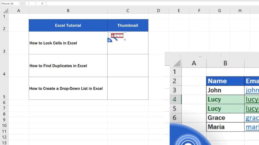
Click anywhere into the blank part of the worksheet area and then on the picture again. The inserted image can now be moved or resized using these little circles on its sides.

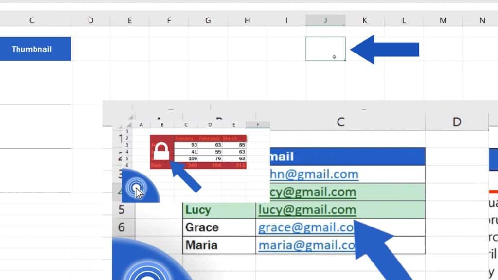
And here’s a small tip to make it all easier.

How to Adjust the Image Size

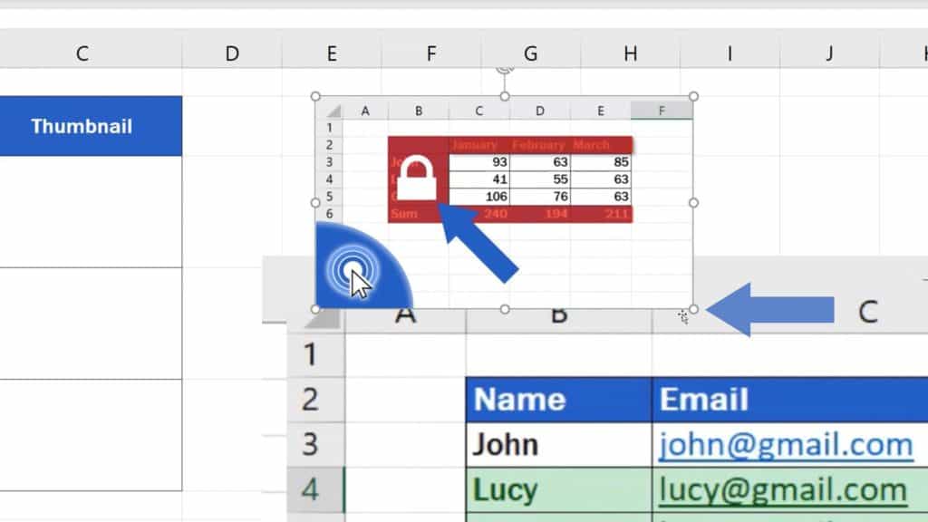
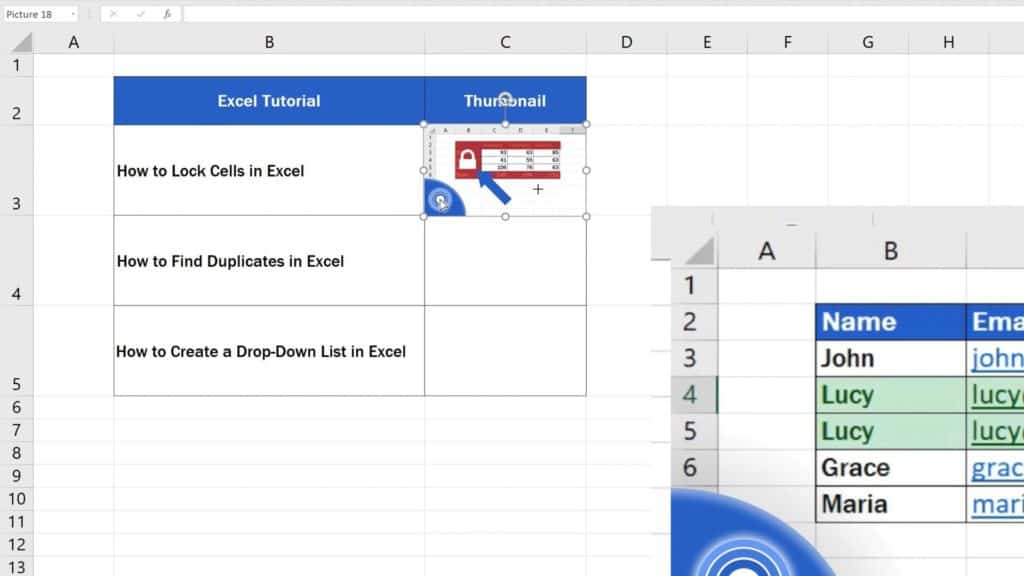
If you need to adjust the image size to the size of the cell spot on, keep the button Alt pressed while dragging the image around. It’ll help you fit the picture into one of the cell corners and align it with its borders with more accuracy.

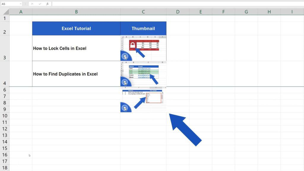
Repeat the steps above to insert the rest of the pictures into the cells, and we’re gonna have a look at one important thing regarding the picture formatting.

How to Hide the Row Contains Inserted Image

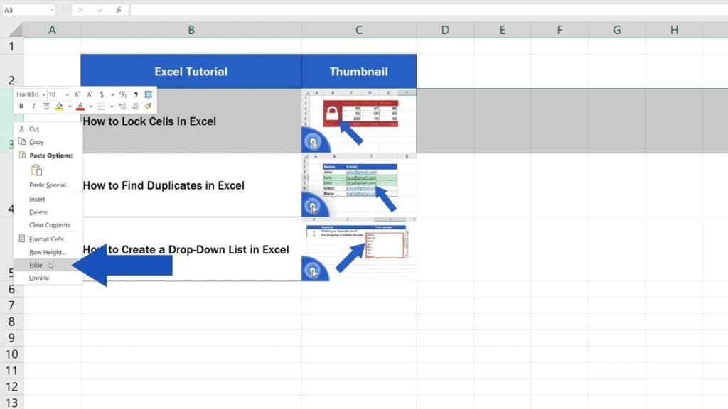
Imagine that now you need to hide a row. Hiding the row itself is not the problem. But if the row contains an inserted image, you’ll see that the picture usually stays visible, which means it gets in your view and covers important data in the spreadsheet. This can make your work disorganised and complicated not only when it comes to hiding rows, but also with filtering or other operations.

The question is: how to deal with that?

Let’s undo the last changes and we’re gonna go through it together.

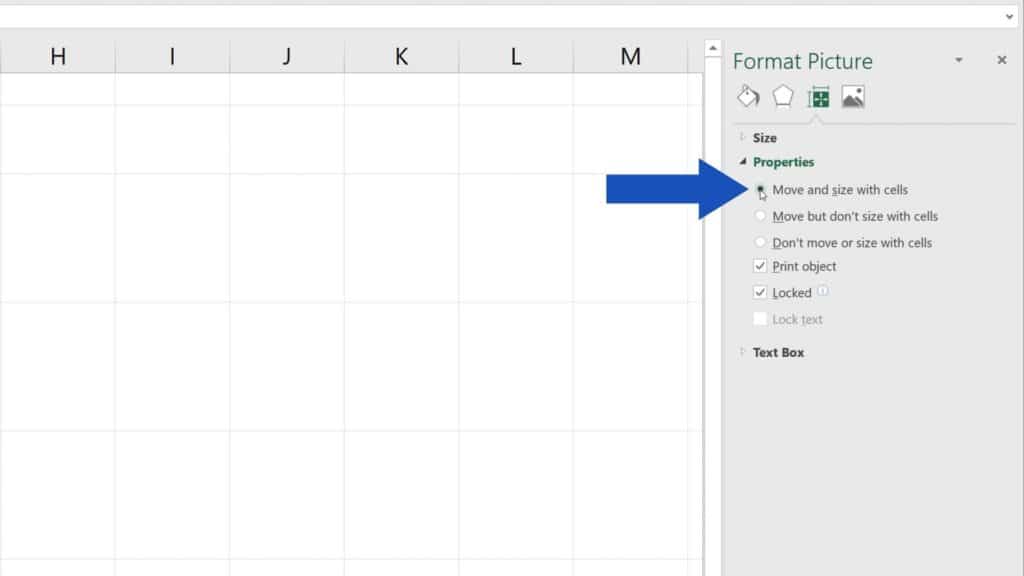
Right-click on the image and choose ‘Format Picture’.

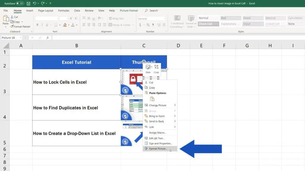
On the right-hand side, a task pane with multiple options appears. Switch to ‘Size and Properties’ tab. Go to ‘Properties’ and select the option ‘Move and size with cells’. This will ensure that the image will move with the target cell. We can check it together right away.

Let’s hide row number 3, which contains the image.

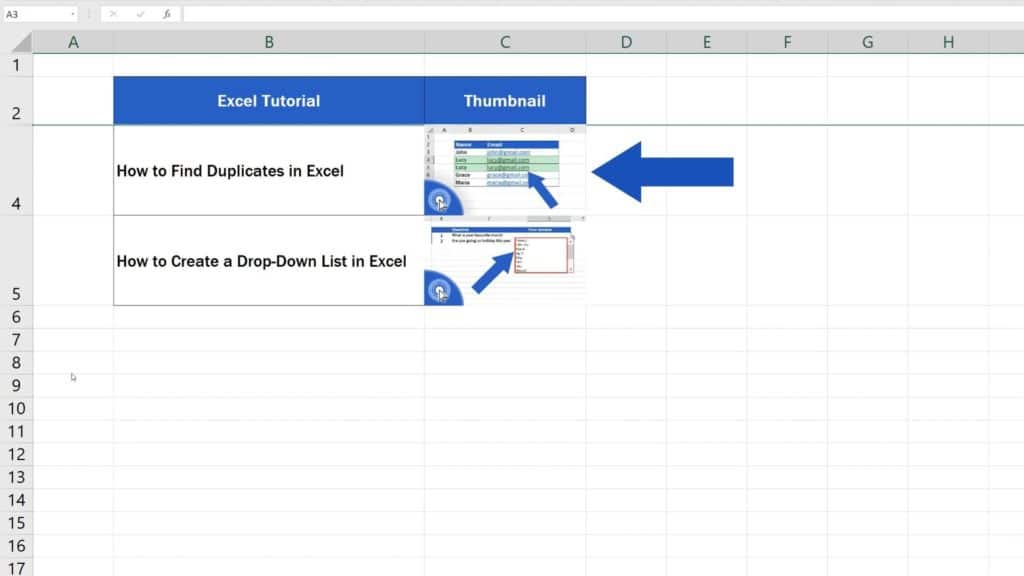
You can see that the picture has also disappeared along with the whole row. Nothing now stands in the way of a neat spreadsheet with all important data well organised.

Are you wondering :

• How to Hide Rows in Excel
• How to Insert Row in Excel

If you found this tutorial helpful, give us a like and watch other video tutorials by EasyClick Academy. Learn how to use Excel in a quick and easy way!

Is this your first time on EasyClick? We’ll be more than happy to welcome you in our online community. Hit that Subscribe button and join the EasyClickers!

Thanks for watching and I’ll see you in the next tutorial!