How To Lock Formulas In Excel

This video tutorial shows the easiest way how to lock formulas in Excel. You’ll be able to protect the formulas in your data table, so that no one will be able to rewrite them, which practically means that the calculations in the table will always be processed the way you need them to be processed and no other way.

Sounds interesting? Let’s try it together!

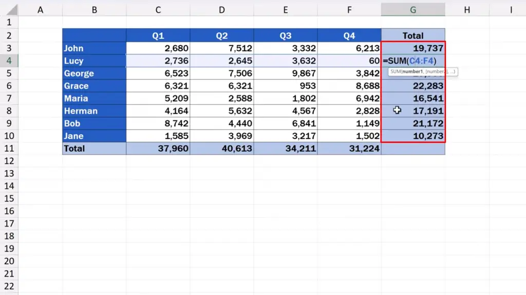
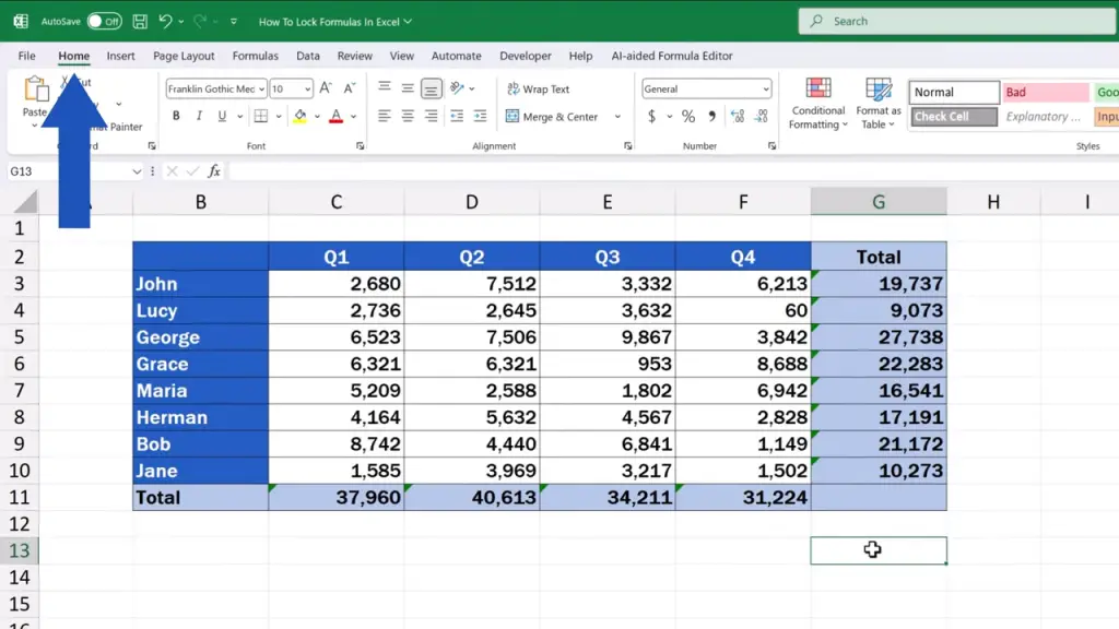
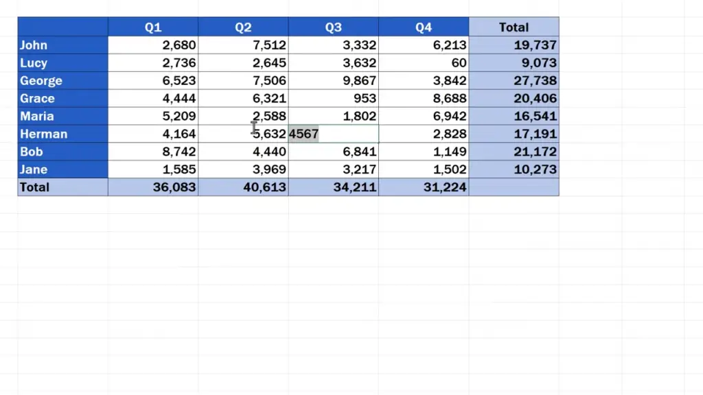
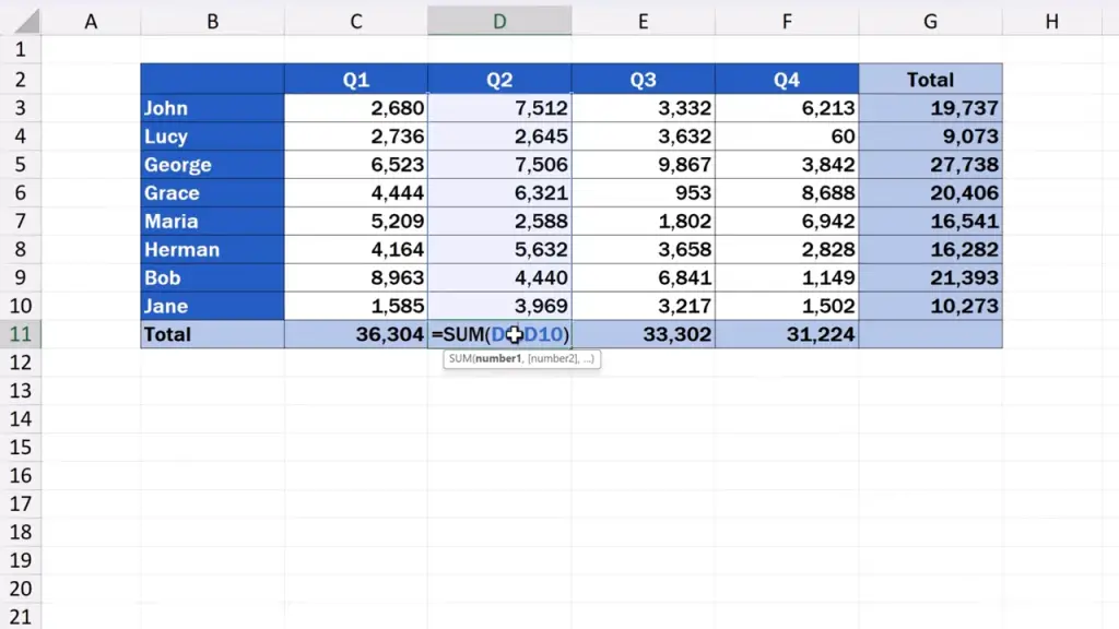
To have a look at the whole process of how to lock formulas in Excel, we’re going to use this data table containing the sales information for each business quarter.

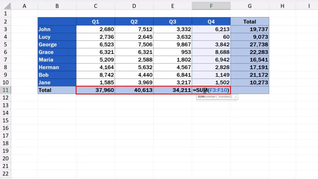
At the same time, it stores formulas that add these figures up in the last column and the last row.

Now, we’re going to lock these formulas, so that no one could change them, but we might want other people to be able to alter some data, so we’ll leave the cells that don’t contain a formula open for editing by anyone.

How to Unlock All Cells Before Locking Formulas

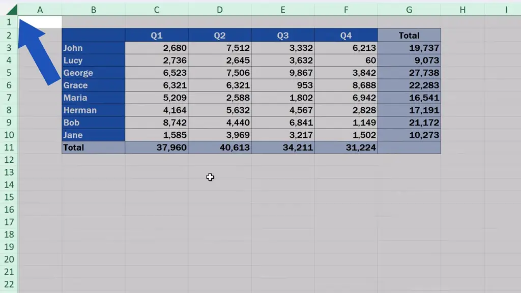
First, we click on the left upper corner of the spreadsheet.

The whole spreadsheet’s been highlighted now.

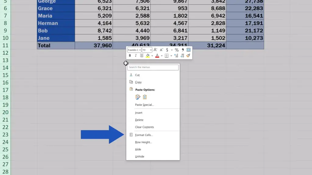
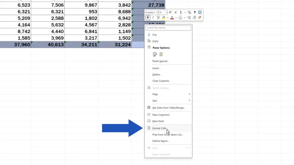
Then we right-click anywhere on the selected area and choose ‘Format Cells’.

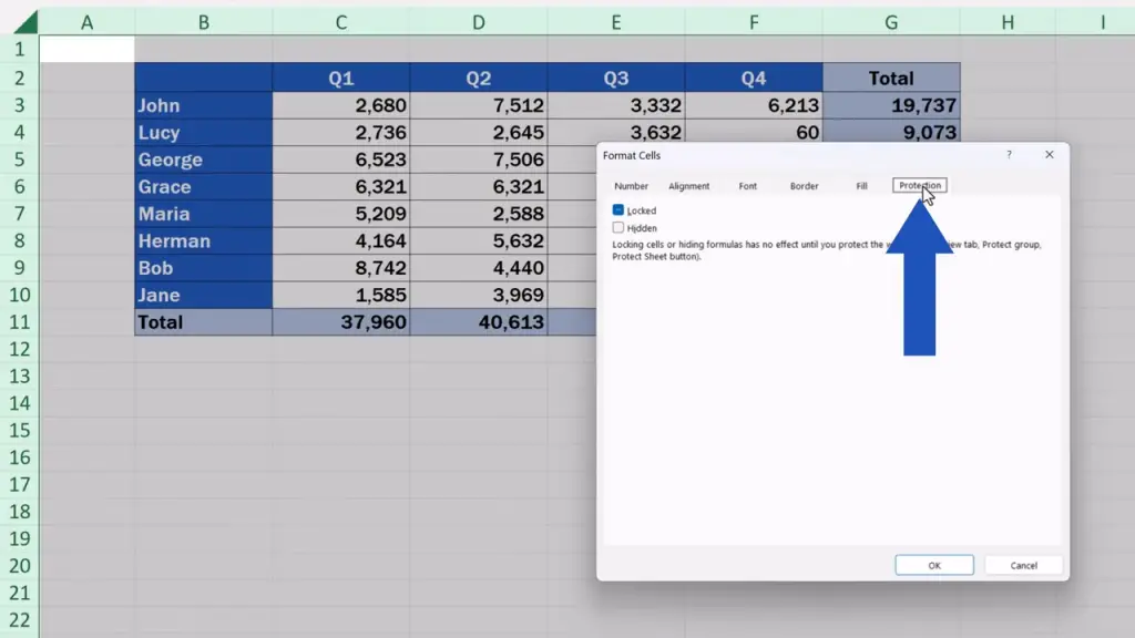
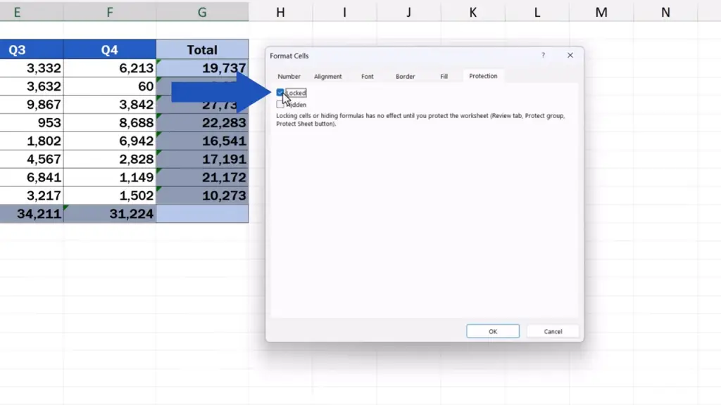
We go to the tab marked ‘Protection’.

And untick this box that says ‘Locked’. We don’t want the box to be selected as an option.

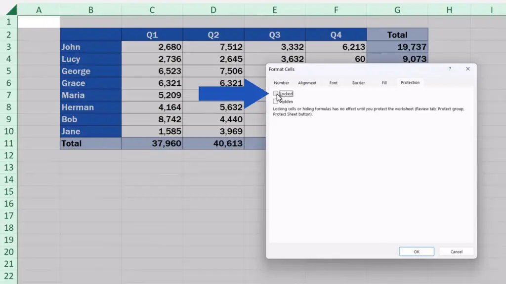
This way we made all the cells in the spreadsheet unlocked, which basically means open for editing.

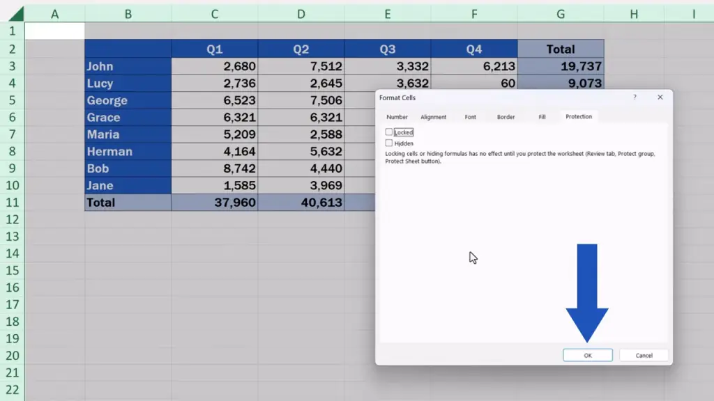
We click on ‘OK’ and move on.

How to Select and Lock Only Formula Cells

Next, we’ve got to select all the cells in the table containing a formula. We can do this in a very simple way, by using the function ‘Go To Special’.

Up in the ‘Home’ tab,

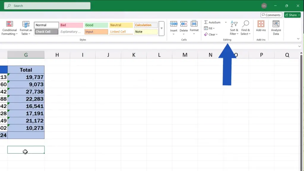
in the section ‘Editing’,

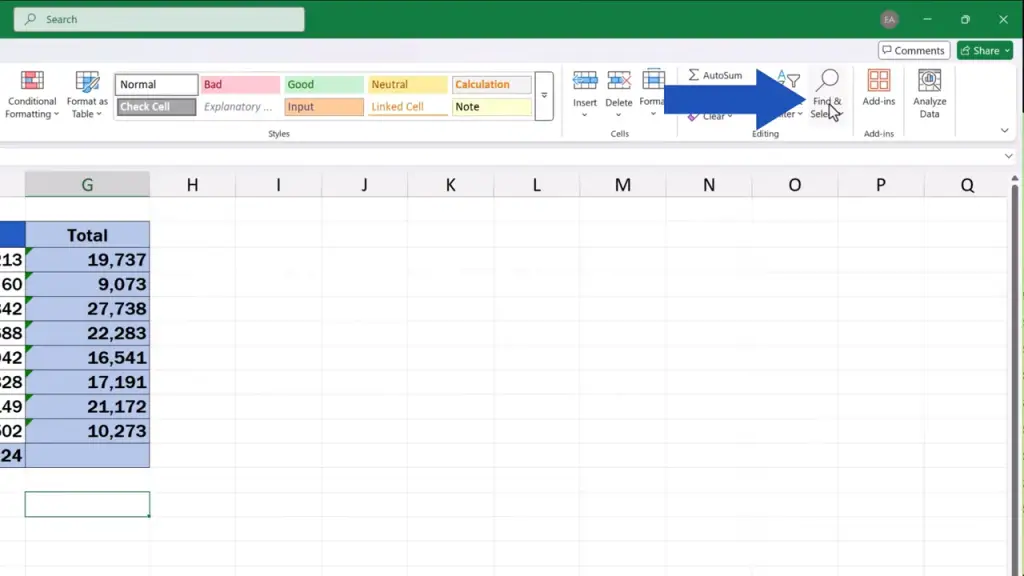
we click on ‘Find & Select’,

then we click on ‘Go To Special’.

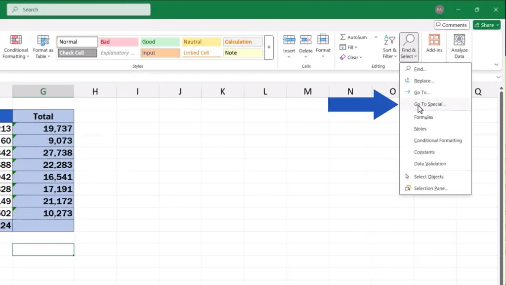
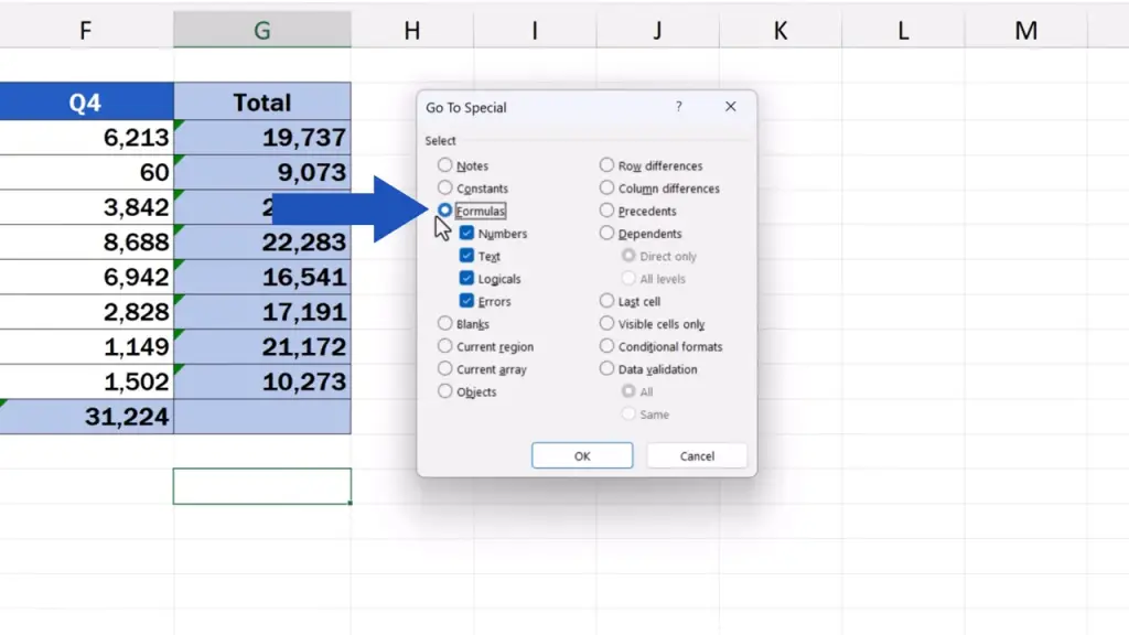
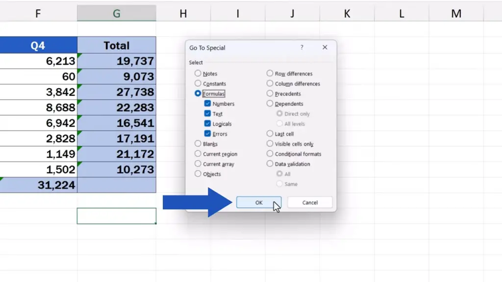
In the window that pops up, we click on ‘Formulas’ and we can keep all the boxes with the four options ‘Number’, ‘Text’, ‘Logicals’ and ‘Errors’ ticked. Excel will then find and select all cells containing formulas, no matter what type of the result they provide.

Now we can click on ‘OK’ and here we go.

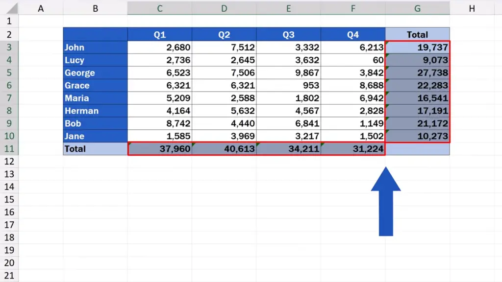
All cells containing a formula have been highlighted!

How to Protect the Sheet to Lock Formulas

And let’s move on to the third step. Now, we can indicate that all these cells with formulas are to be locked.

We right-click on the selected cells

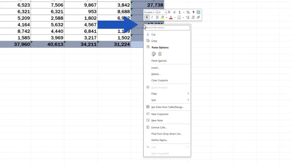
and we click on ‘Format Cells’ again.

When we go to the ‘Protection’ tab, we now tick the box ‘Locked’.

This means we want to lock these selected cells for editing. We click on ‘OK’ and here’s the last thing to be done.

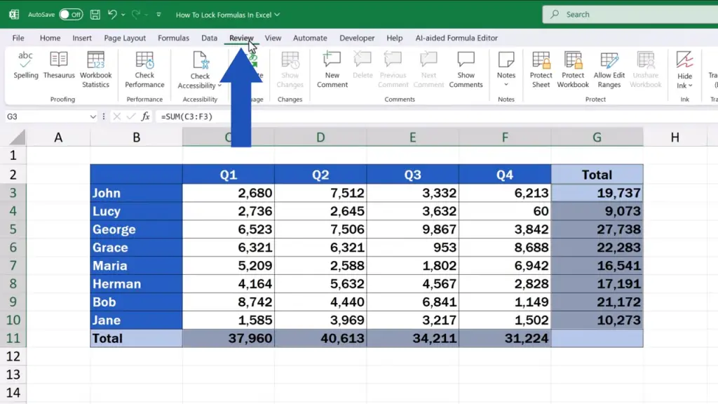
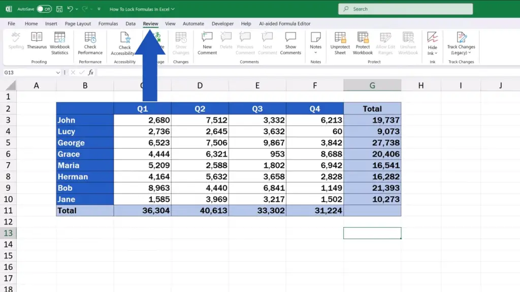
To make the settings work, we need to ‘activate’ the lock. So, we click on the ‘Review’ tab

and go to ‘Protect Sheet’.

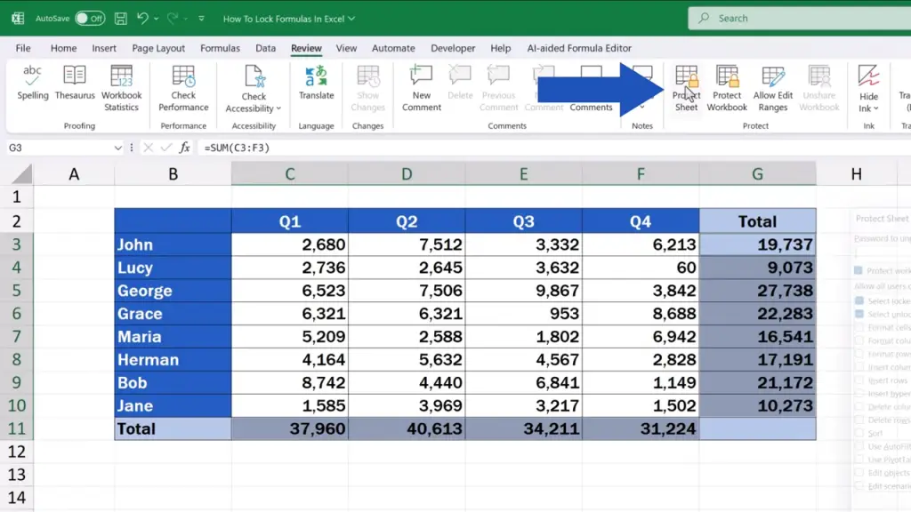
Here we can set a password for protection if needed or specify what exactly other users will be allowed to do with the locked cells.

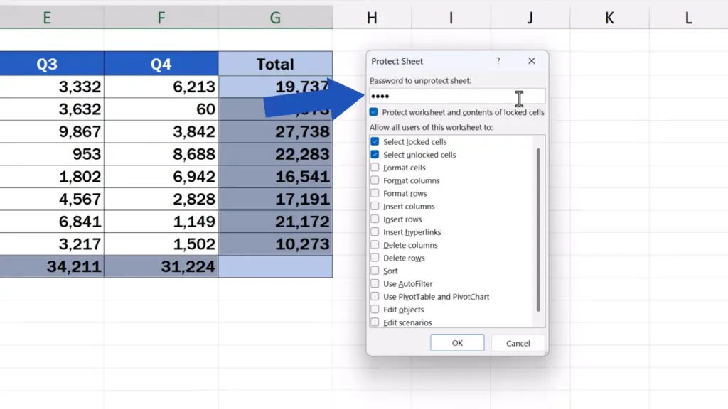
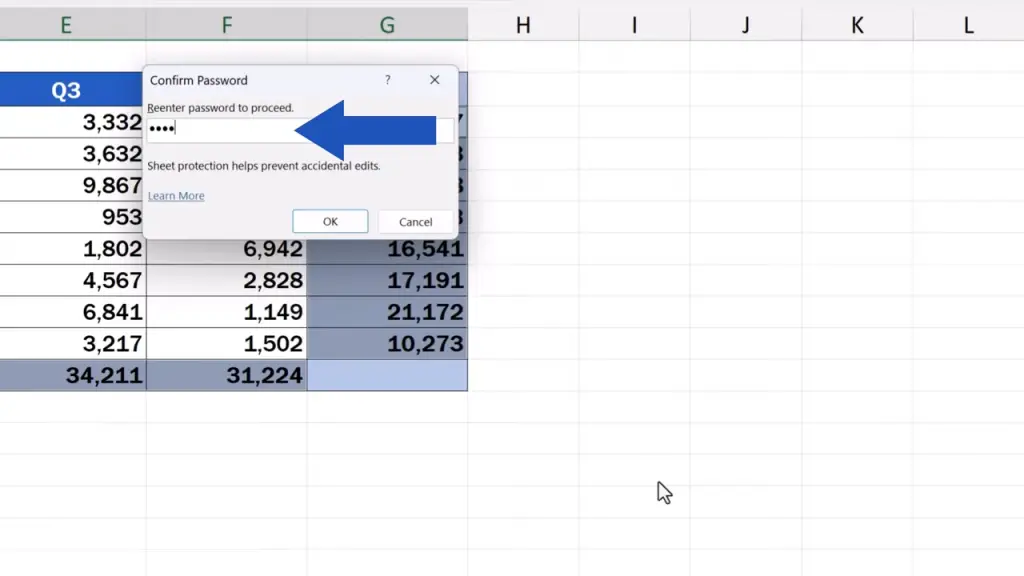
In this case, we’re going to set a password and leave the rest as it is.

All cells containing a formula have now been locked and protected, other cells have been kept open for editing and we’re going to check this right away.

If we click on a cell containing a sales figure, Excel allows us to rewrite it.

But if we click on any cell that contains a formula, Excel won’t let us do anything and a notification will show that the cell’s locked.

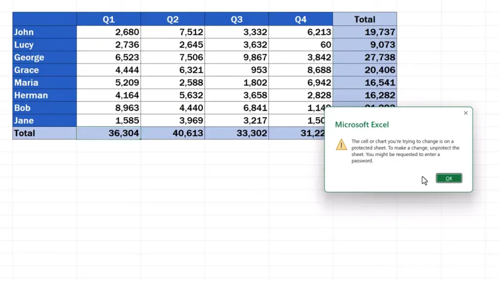
So, everything’s working as it’s supposed to.

How to Unprotect a Sheet in Excel

If cell protection is no longer needed in the sheet and you want to remove it, that’s also a very easy thing to do.

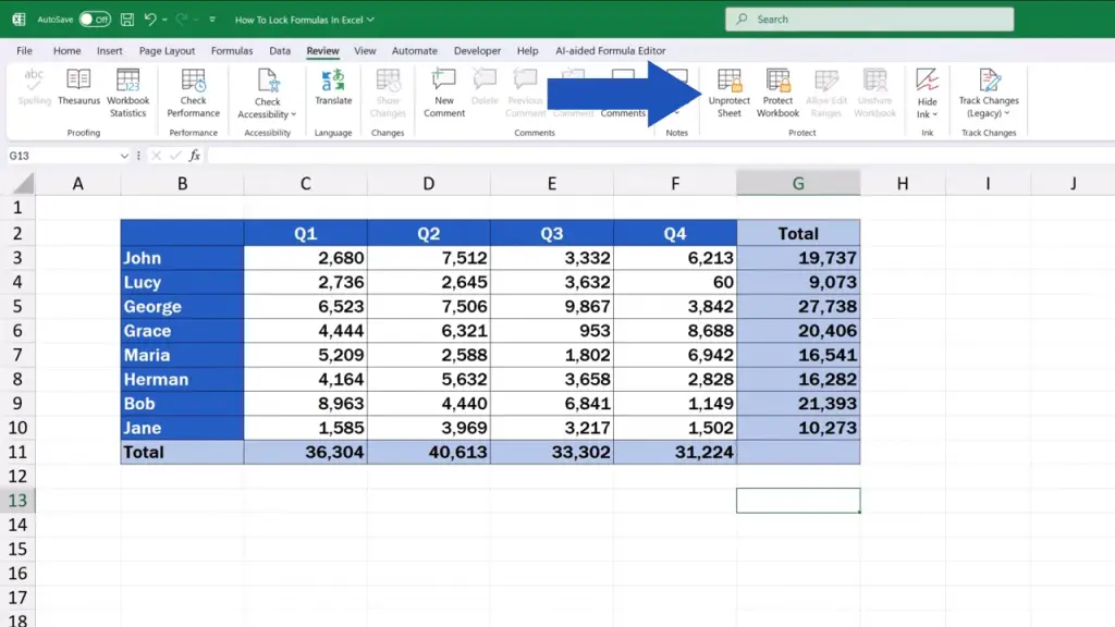
Simply, go back to the ‘Review’ tab

and click on ‘Unprotect Sheet’.

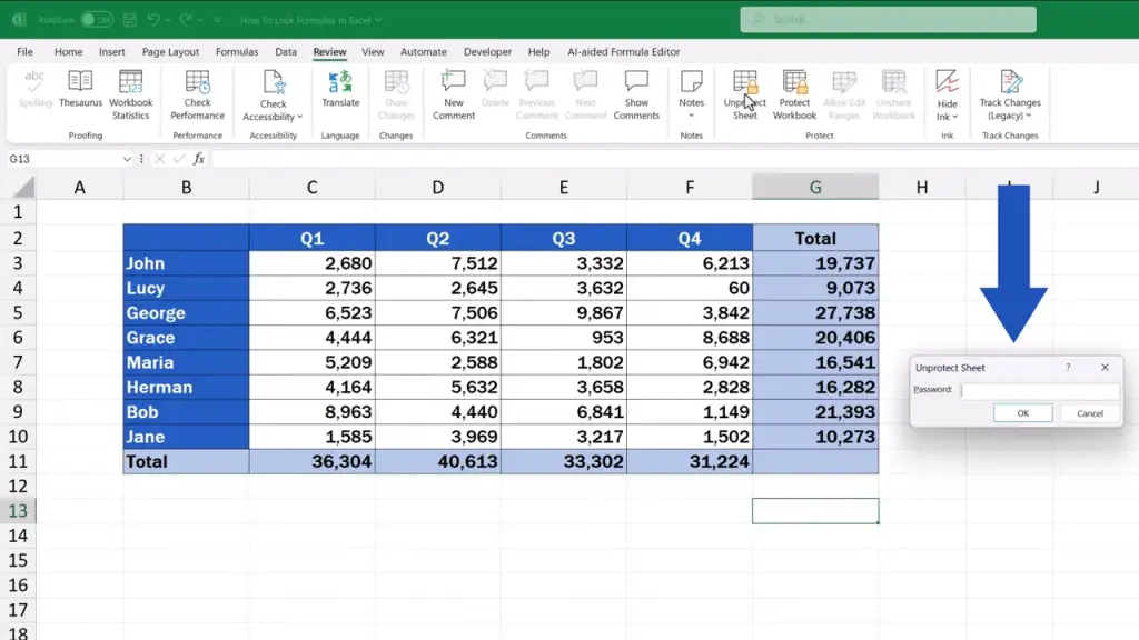
If you’ve set a password, you’ll need to enter it now. If not, the sheet will get unprotected right away.

And we’re done for the day!

This way you can protect formulas in data tables against an unwanted intervention and the data tables will always be working according to what you need.

Don’t miss out a great opportunity to learn:

• How to Apply a Formula to an Entire Column in Excel
• How to Copy a Formula Down a Column in Excel

If you found this tutorial helpful, give us a like and watch other tutorials by EasyClick Academy. Learn how to use Excel in a quick and easy way!

Is this your first time on EasyClick? We’ll be more than happy to welcome you in our online community. Hit that Subscribe button and join the EasyClickers!

Thanks for watching and I’ll see you in the next tutorial!