How to Make a Pie Chart in Excel

In this tutorial, you’ll see how to create a simple pie graph in Excel. Using a graph is a great way to present your data in an effective, visual way.

Let’s have a look, then!

See the video tutorial and transcription below:

See this video on YouTube: 
https://www.youtube.com/watch?v=hElkEzAjd5o

Excel offers many different chart types and choosing just the right kind of graph can make your data presentation clear and engaging. In the previous tutorials, we learned how to make a line graph

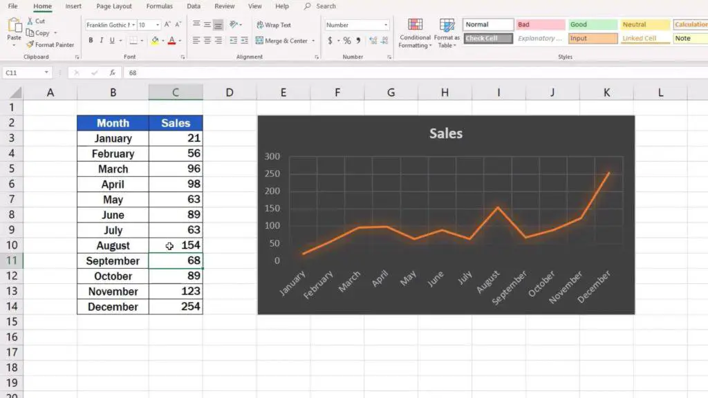
and also bar graph.

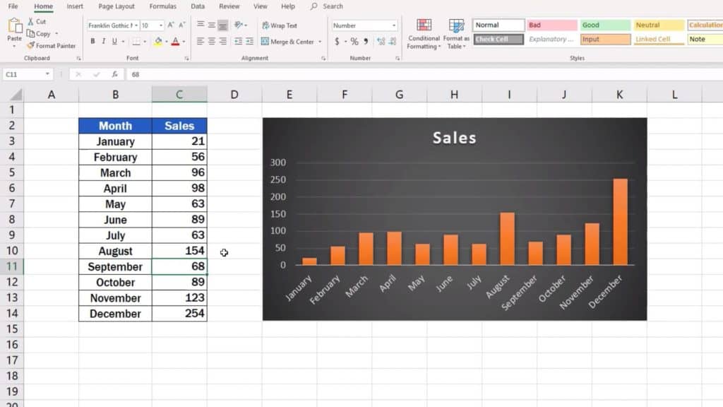
In this tutorial, we’ll take some time to explore the pie chart, specifically, how to use it to present monthly sales, which you can see in this table .

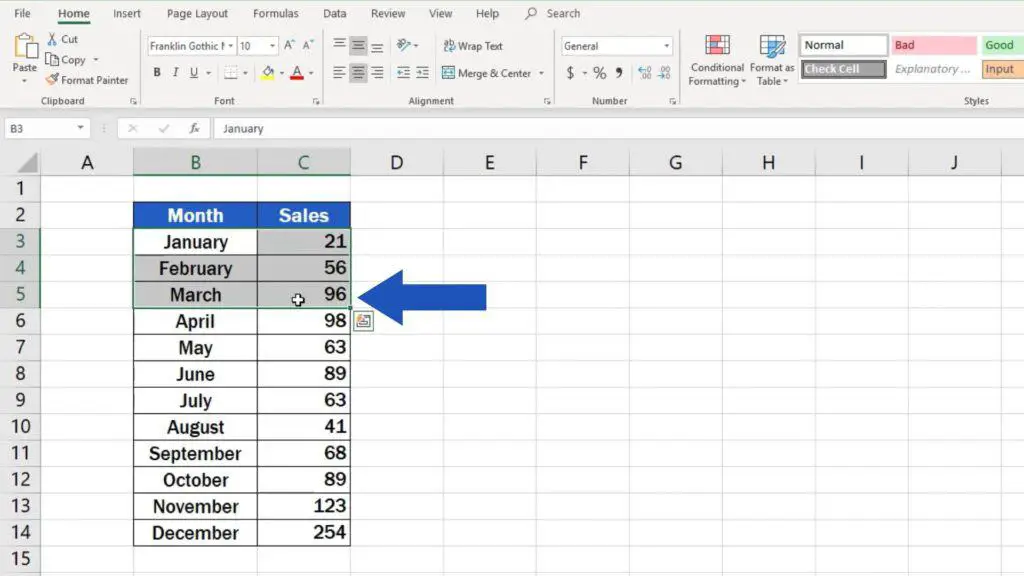
First of all, as usual, we need to select the area with the relevant data – the data we want to present in the graph.

Click on the ‘Insert’ tab, go to section ‘Charts’ and select the pie chart option.

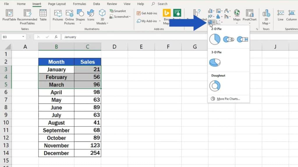
There are more chart design options to choose from, but for now, we’ll pick the first one.

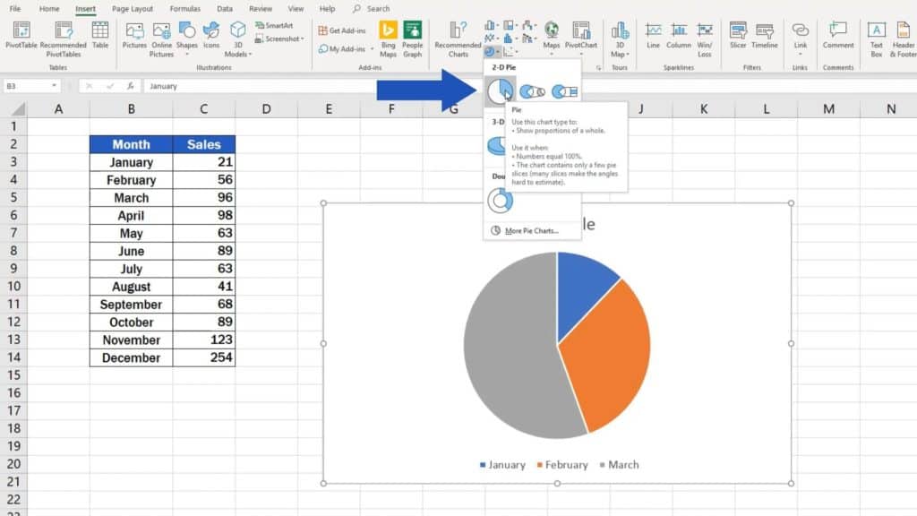
Excel will immediately draw the chart and insert it in the spreadsheet.

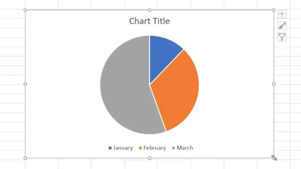
Now, let’s see what we can do to improve the chart or customise it more to our liking.

How to Adjust the Position of the Chart Within the Excel Spreadsheet

The position of the chart within the spreadsheet can be adjusted in a very simple way. Click on the blank space within the chart area, hold the left mouse button and move the graph any direction to place it exactly where you need.

How to Adjust the Size of a Pie Chart in Excel

You can easily adjust the size of the chart, too – simply by clicking into any corner of the chart area, on one of the little circles, and dragging any direction until the size of the chart is just what you need it to be.

Let’s move on!

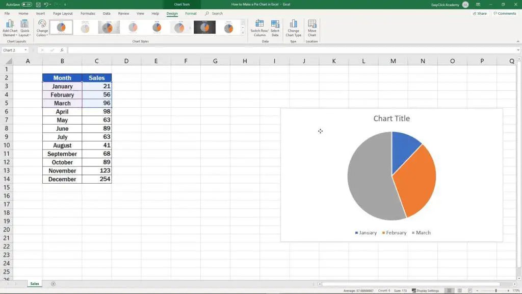
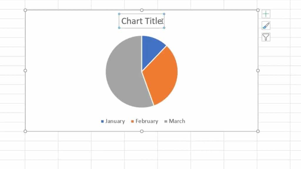
How to Add a Chart Title in Excel

The title of the graph now contains the caption ‘Chart Title’. Of course, you can name your pie chart anything you want. Just click on the caption to make it editable and type in your own title.

And we’re still not finished here!

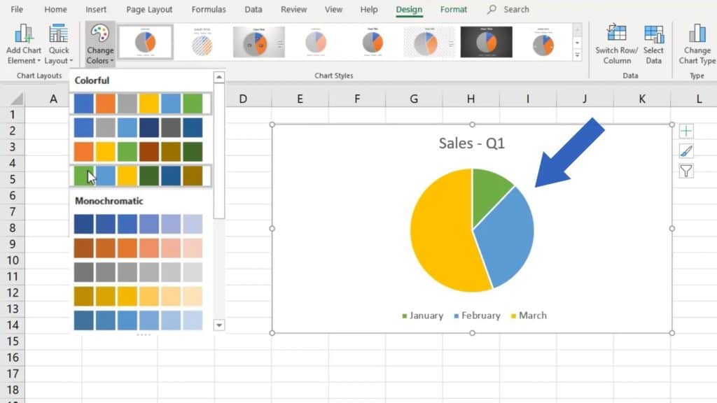
How to Change Colour and Design of the Chart

The colour and design of the chart can also be easily changed according to your preference. Click on the blank space of the chart area again, go to ‘Design’ tab and find the option ‘Change Colour’ to pick from a selection of colours.

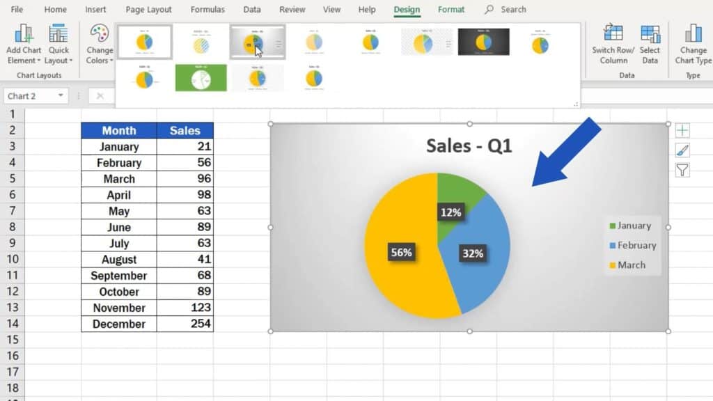
In addition, the whole graph design can be changed in a similar way. Go to ‘Design’ tab once again, look for ‘Chart Styles’, click on the drop-down arrow and you’ll see a list of options to choose from. You can select the style that suits you best.

And here’s one more thing before we finish.

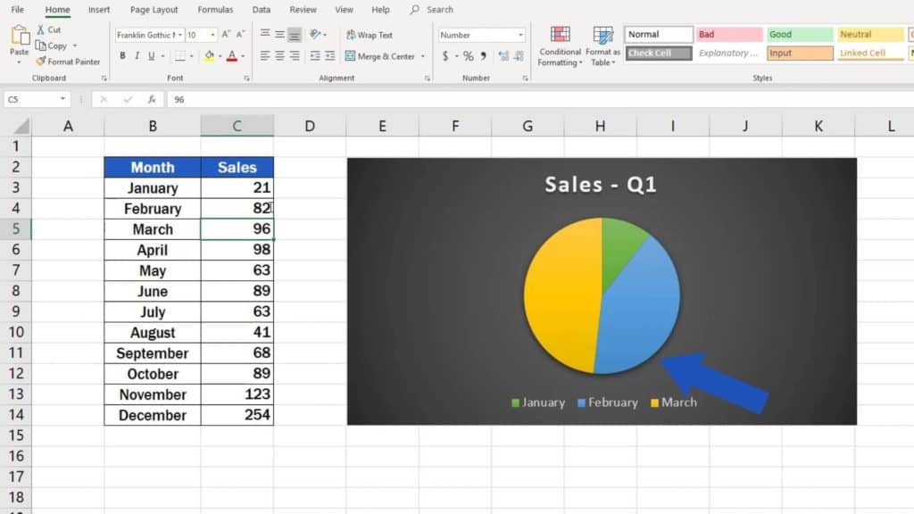
A graph in Excel is dynamic, which means that if you change any data in the source table, it will be reflected in the graph, too. For example, we’ll change the sales figure for February  from 56 to 82. The chart has automatically updated to show this new value.

If you’re interested in learning more about other types of graphs or how to improve already created charts, watch the upcoming EasyClick Academy tutorials!

Don’t miss out a great opportunity to learn:

• How to Make a Line Graph in Excel
• How to Make a Bar Graph in Excel
• Try out Data Bars in Excel for clear graphical data representation

If you’re curious how you could make the design of your data tables even more effective, watch more video tutorials by EasyClick Academy!

• How to Use Color Scales in Excel (Conditional Formatting)
• How to Merge Cells in Excel
• How to Wrap Text in Excel
• How to Change Text Direction in Excel

If you found this tutorial helpful, give us a ‘like’ and watch other video tutorials by EasyClick Academy. Learn how to use Excel in a quick and easy way!

Is this your first time on EasyClick? We’ll be more than happy to welcome you in our online community. Hit that Subscribe button on our YouTube channel and join the EasyClickers!

See you in the next tutorial!