How to Multiply Numbers in Excel (Basic way)

This tutorial will guide you through a simple way how to multiply numbers in Excel.

Here we go!

See the video tutorial and transcription below: 

See this video on YouTube:
https://www.youtube.com/watch?v=C5XMaKUhcEE

Basic Way How to Multiply Numbers in Excel

To start with, it’s important to realise that there’s more than one way how to do multiplication in Excel, and these methods are more advanced. Here we’re gonna concentrate on the basic, simple way how to multiply two numbers in a table.

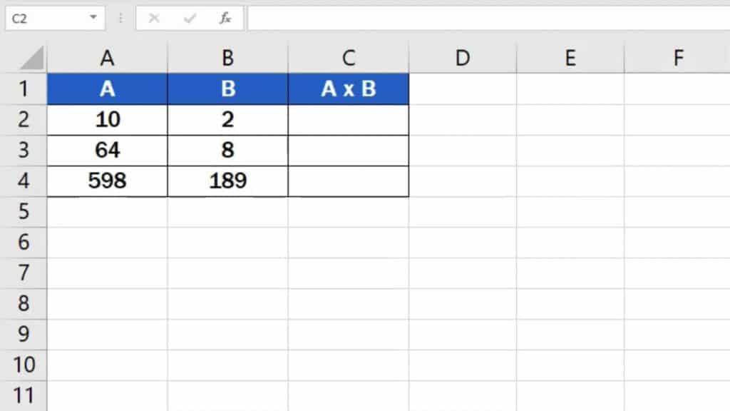
We’ll use this table as an example to show how to work out anything we need, step by step. There are numbers written in columns A and B. Thanks to an easy formula, we’ll multiply them and the result will appear in column C.

First, click on the cell in which you want to display the result. Let’s select cell C2 for our first calculation.

Now, find the ‘equal’ key and press it. This works as some kind of signal to Excel that we want to enter a formula in the cell.

Then we click on the cell that contains the first number to be multiplied, in this case, it’s cell A2. Once we’ve selected the cell, we can see how another part of the formula appeared after the ‘equal’ sign – it’s the cell reference, A2.

Next, we need to add the symbol for the mathematical operation we want to carry out, so we’ll use an asterisk, which is used for multiplication in Excel.

After that, click on the cell which contains the multiplier, which is B2.

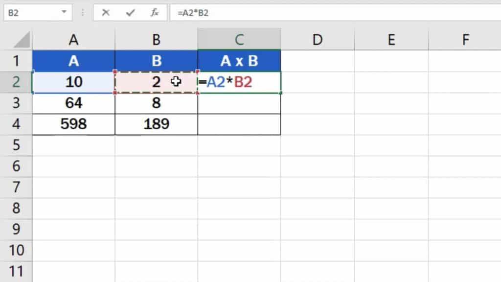
So, what we’ve just done is that we’ve told Excel to multiply the number in cell A2 with the number in cell B2.

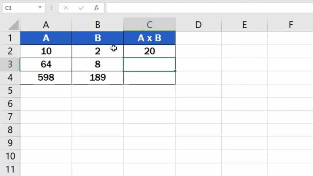
Hit ‘Enter’ and you’re done! The result is available at once.

You can use similar steps to add, subtract or even divide in Excel. You can watch separate tutorials that describe how to do these calculations in more detail.

But this is not all! Here comes a handy little ‘lifehack’ just for you!

How to Copy Formula into Adjacent Cells by Using the Fill Handle

If you need to multiply the numbers in rows 3 and 4, click on the cell containing the formula we’ve just created, which is cell C2.

Hover over the bottom right corner of the cell until you see a cross symbol, then use left-click to drag the formula down through the rest of the rows.

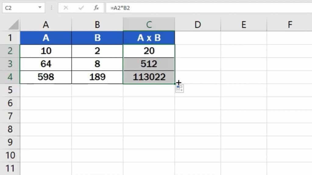
And that’s it! Well done! You’ve managed to multiply the numbers in all three rows!

Are you wondering:

• How to Calculate Hours Worked in Excel
• How to Add Numbers in Excel (Basic way)
• How to Subtract Numbers in Excel (Basic way)
• How to Divide Numbers in Excel (Basic way)

If you’ve found this tutorial helpful, like us and subscribe to receive more videos from EasyClick Academy. Look at more tutorials that help you use Excel quick and easy!

See you in the next tutorial!