How to Refresh a Pivot Table in Excel

Pivot tables are amazing tools to summarise and analyse data. But as soon as anything changes in the source data, we’ve got to refresh them to keep them up to date. This video tutorial offers an ultimate guide on how to refresh a pivot table in Excel to make sure the pivot table shows the right, most up-to-date data.

Ready to start?

How to Refresh a Pivot Table After Changing a Value

When working with pivot tables, we must keep in mind that if anything changes in the source data, it won’t automatically show in the pivot table.

Let’s have a look at how it actually works.

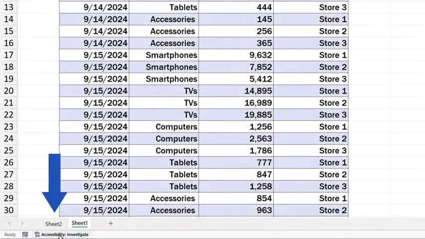
We start with clicking into Sheet1, which contains our source data .

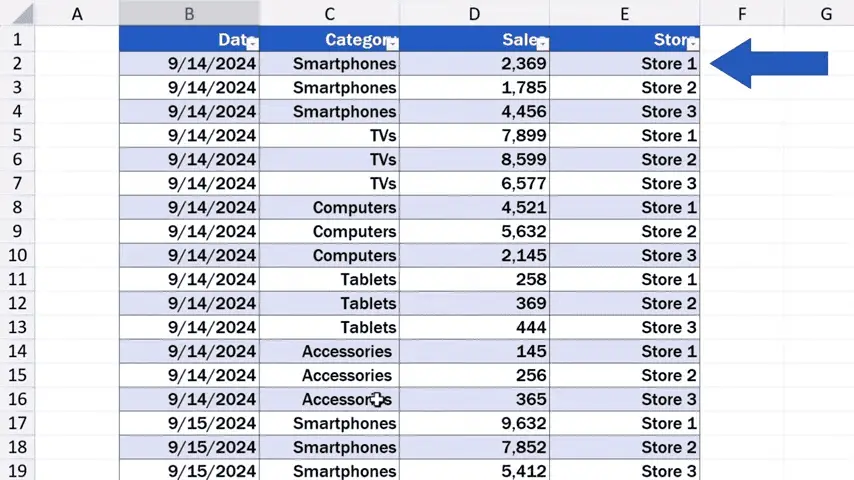
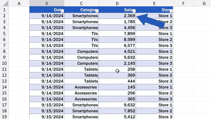
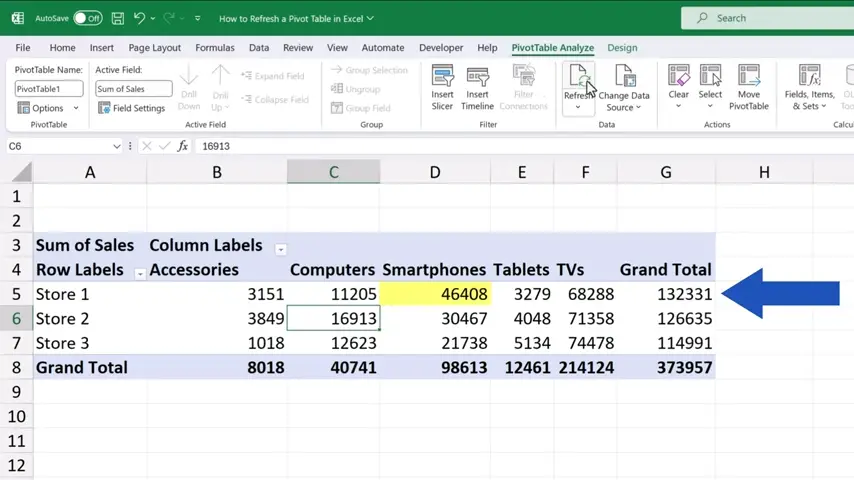
And we rewrite this number, which is the value of the sales for Store 1 in the category ‘Smartphones’, to 15,000 USD.

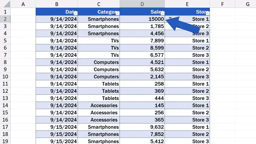
If we go back to Sheet2, which contains our pivot table, we can see that it shows no change in values.

That’s why we’ve got to refresh the pivot table and this is how we do that.

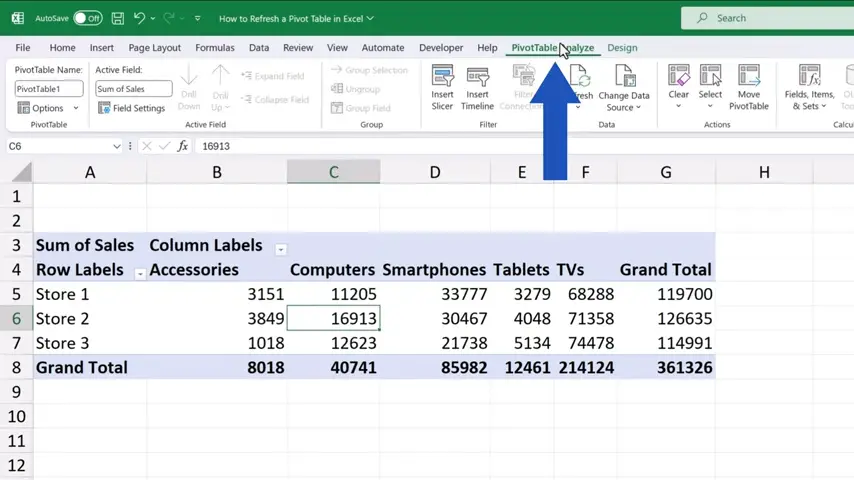
We click anywhere in the pivot table, so that the PivotTable tab appears.

There we click on ‘Refresh’ and that’s it!

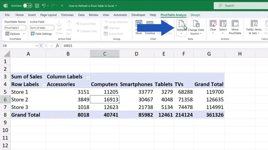
Excel has updated the pivot table with the most up-to-date sums.

So, if you simply rewrite a value in the source data, you can just refresh the pivot table and you don’t have to do anything else. However, adding new rows or columns, which basically changes the source data range, might be a bit trickier.

We can take a look at how to deal with this more advanced source data update, now.

How to Check the Pivot Table’s Data Source

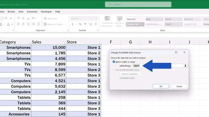
Let’s start with a very important detail – the way the pivot table pulls data from the source, because that can have a great impact on the result. This we can check by clicking anywhere within the pivot table area and finding the option ‘Change Data Source’ in the PivotTable tab.

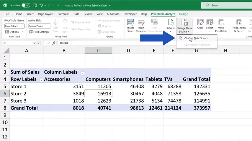
Here we can see whether the data source is a table or a directly specified range of cells.

Here it says ‘Table’, which makes it easier to add a row or a column if needed, because with tables, Excel automatically updates the source range.

But if the field contains a manually entered range, it’ll need to be updated manually every time a row or a column is added.

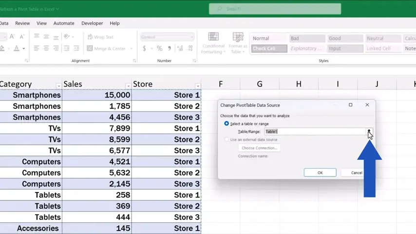
That’s why it’s useful to prepare and organise the source data effectively and format them as a table in advance.

We’re not going to change the range here, because we want to use the table that’s already been specified in the field. So, we can press ‘Cancel’ and move on.

How to Add New Data to a Pivot Table Using a Table

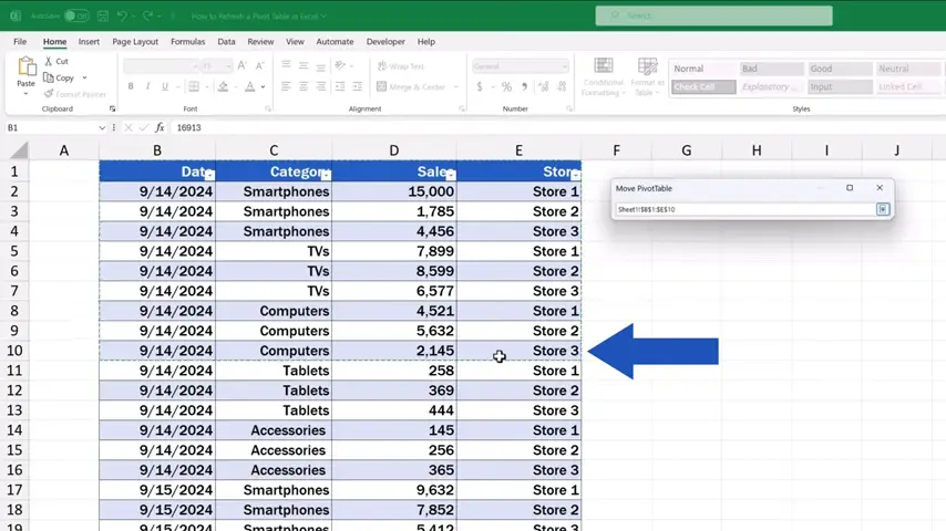
We’ll now click back into our source data and have a look at the benefits of having the data formatted as a table.

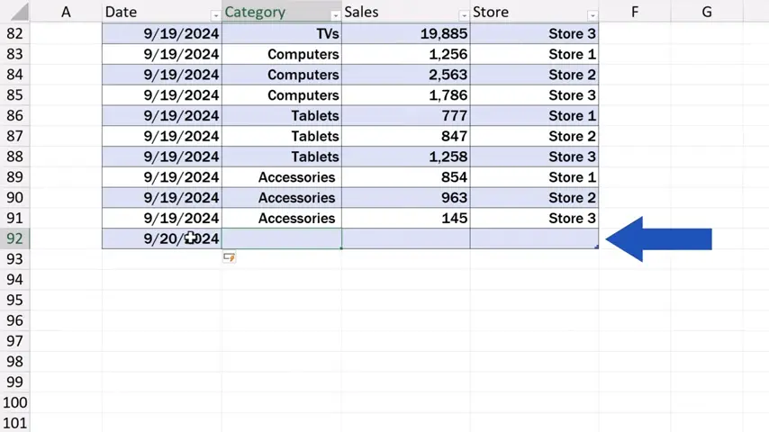
Let’s say we want to add a new row with new data at the very end of the table.

So, we’ll add one with the date 20^th September 2024 and here we go – Excel automatically includes the new row within the original table. This means that the range from which our pivot table pulls data has been updated. When you’ve formatted the source data as a table, you can add as many rows or columns as you like, and you can always be sure that the range for the pivot table is defined correctly.

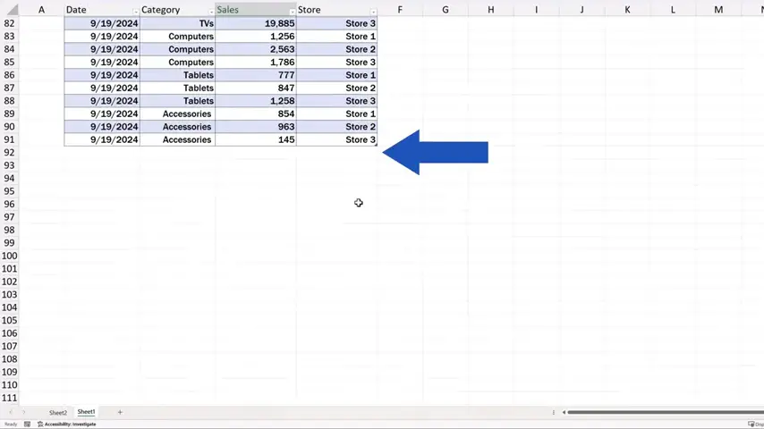
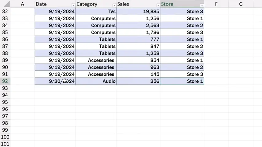
After we’ve added a new row, we can now add a completely new category, for example ‘Audio’, and we’ll be able to watch how this gets reflected in our pivot table later on.

The same way works if we need to delete rows or columns. Let’s delete these rows and see how the table area with the data range changes immediately.

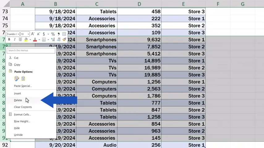
This shows that it actually matters whether we have the source data formatted as a table or entered manually as a range.

How to Refresh a Pivot Table Using the Right-Click Menu

So, we’ve made several changes to our source data and we can click back to Sheet2 which contains our pivot table and this we’ve got to refresh the way you already know.

Now, we won’t use the button up here, but we click anywhere within the pivot table area, then we right-click and look up ‘Refresh’ in the list of options here.

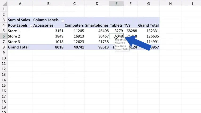
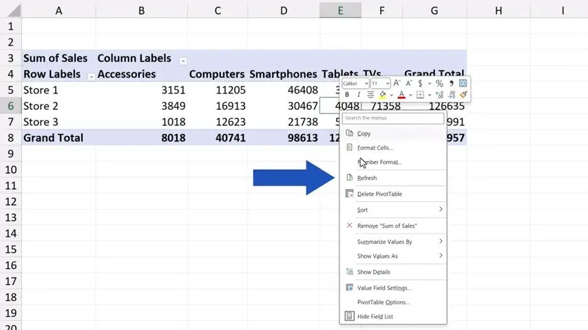
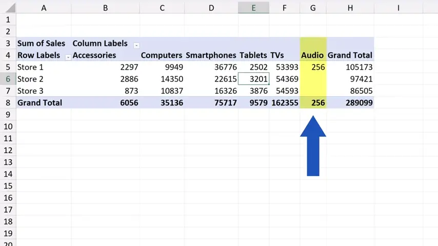
And that’s all it takes! The pivot table has clearly been refreshed, because now we can see the new category ‘Audio’ added a while ago to the source data.

How to Automatically Refresh a Pivot Table When Opening a File

And before we finish, let’s take a look at one more way to refresh the pivot table. This one works automatically, but there’s a catch.

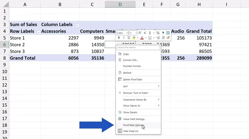
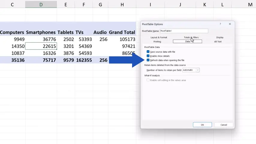
So, click anywhere within the pivot table, then right-click and on the list, find ‘PivotTable Options’.

Move the window aside a bit and click on the tab ‘Data’.

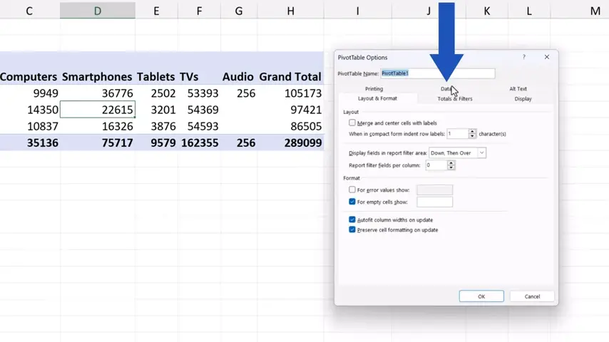
Here we can tick the option ‘Refresh data when opening the file’.

Although it might seem quite practical, that’s also the actual catch – that the data will be refreshed only after you’ve opened the file.

However, any time you open the file, you can be sure your pivot table is up to date.

Don’t miss out a great opportunity to learn:

• How to Create a Pivot Table in Excel

If you found this tutorial helpful, give us a like and watch other tutorials by EasyClick Academy. Learn how to use Excel in a quick and easy way!

Is this your first time on EasyClick? We’ll be more than happy to welcome you in our online community. Hit that Subscribe button and join the EasyClickers!

Thanks for watching and I’ll see you in the next tutorial!