How to Remove Dollar Sign in Excel

This video tutorial offers a quick and easy guide on how to remove the dollar sign in Excel. We’re going to have a look at two different scenarios, so you’ll see what to do if the dollar sign has been entered as part of formatting and how to remove the sign if it’s part of text.

Shall we start?

How to find out whether the dollar sign is part of formatting or text

To remove the dollar sign when used with a number in Excel, we first need to find out whether this symbol shows in the cell because it’s part of its formatting or whether it’s been manually entered next to the number as text.

And that’s actually an easy task to do.

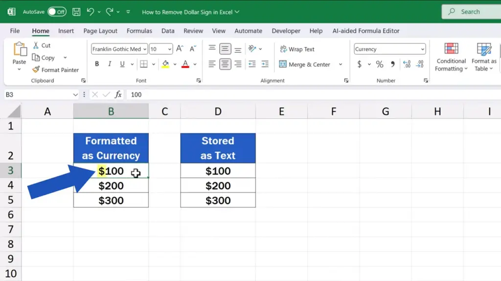
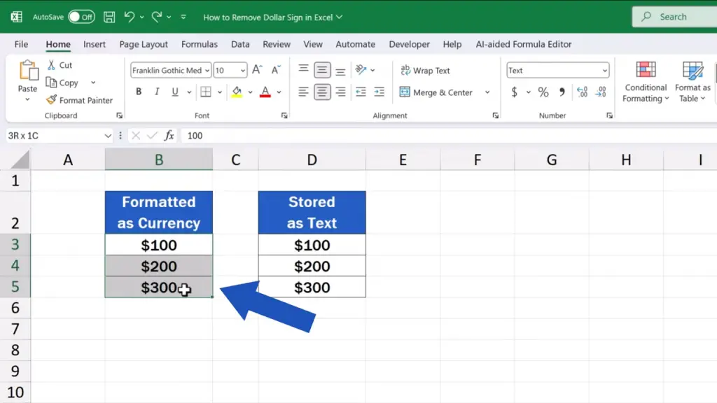
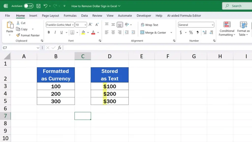
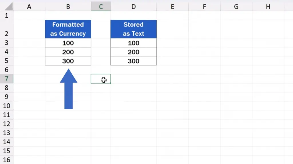
For example, we click on the cell B3

And up here, in the formula bar, we see only the number ‘100’.

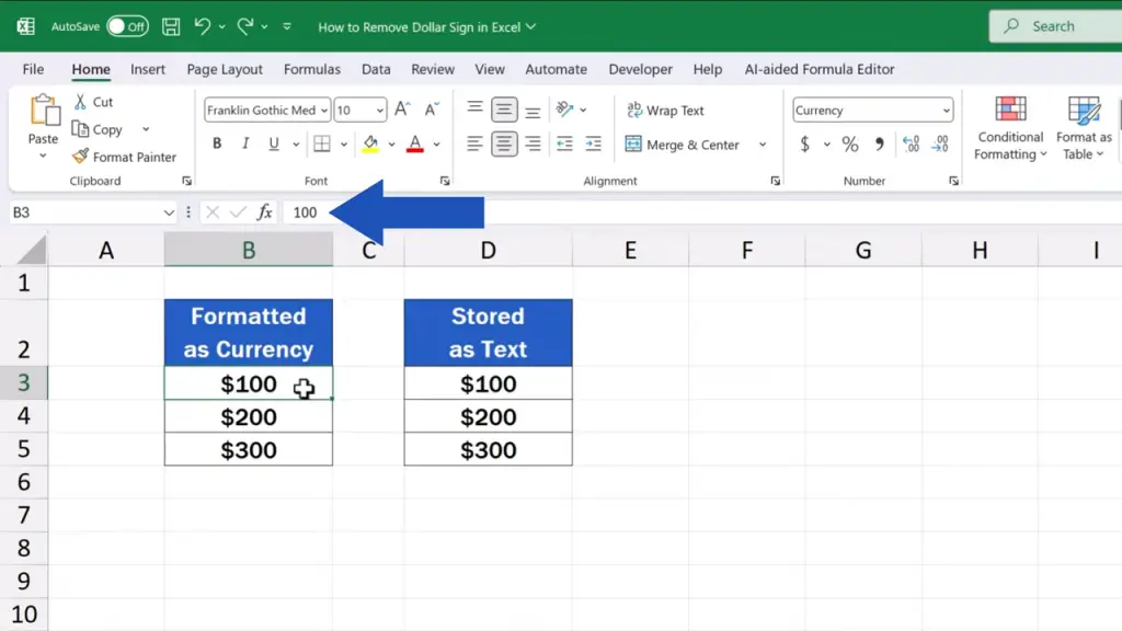
That means the dollar sign here is not part of the value stored in the cell – it’s part of the formatting.

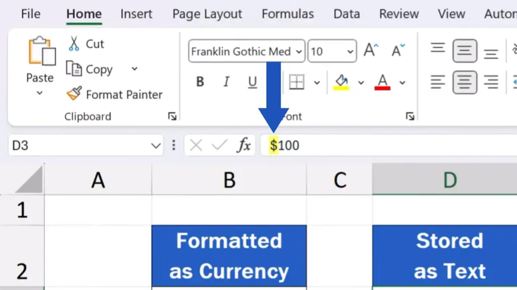
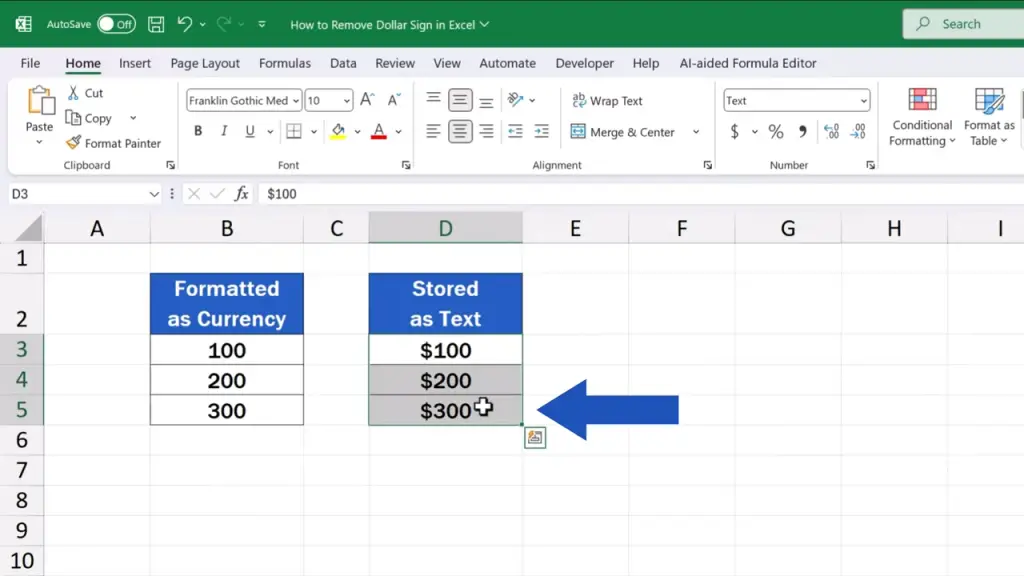
Now, when we click on D3.

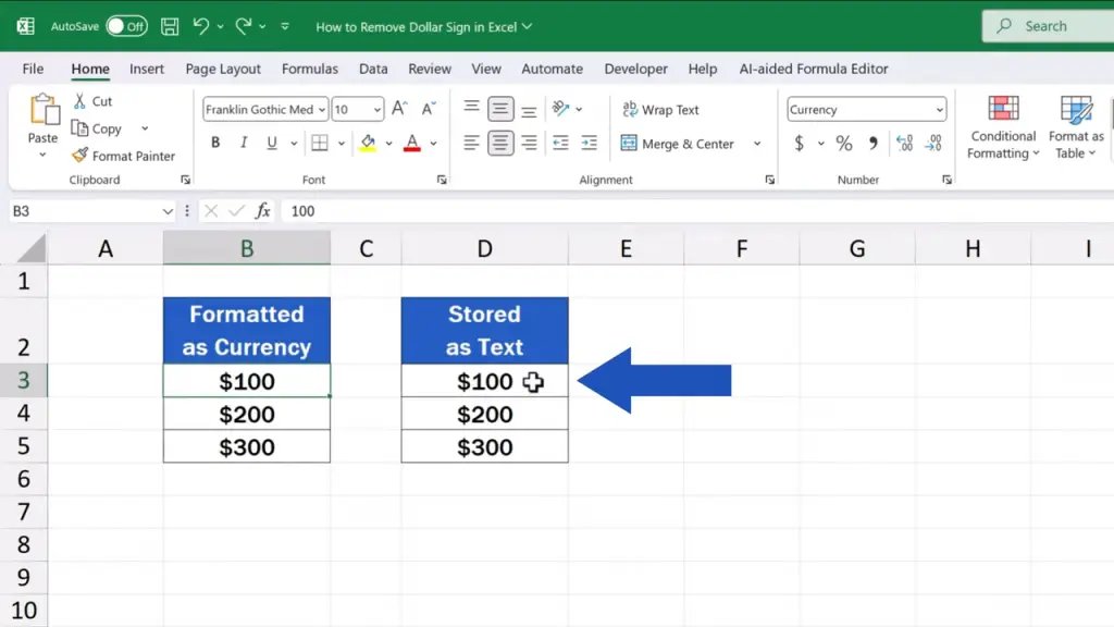
And check the formula bar up here, the dollar sign appears next to the number, which means that the symbol has been typed in the cell manually and it’s stored there as text.

How to remove the dollar sign when it’s part of formatting

Let’s now have a look at how we can remove the dollar sign in both cases.

If the dollar sign is part of formatting, we need to select the cell or cells where we want to remove this symbol, so here we select these three cells.

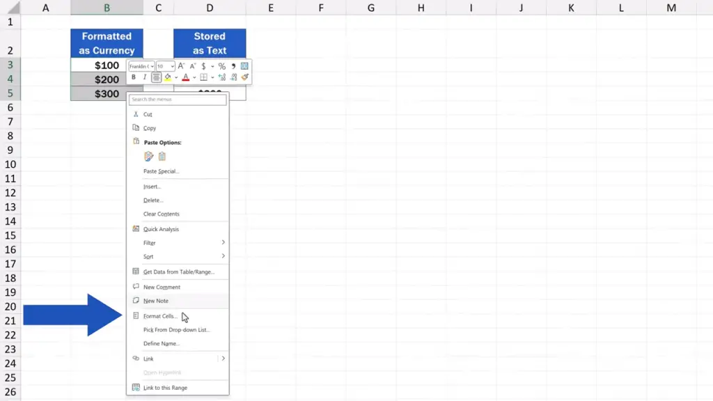
We then use a right click to get to a menu where we look up ‘Format Cells’.

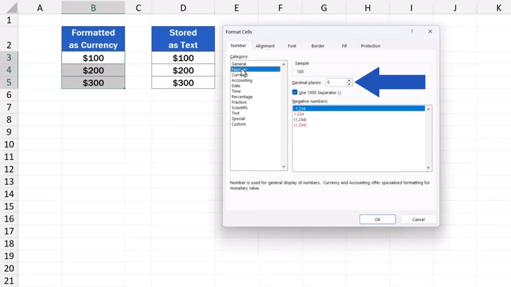
A window appears which we move aside a bit, and we can see that the cells containing these numbers have been formatted as ‘Currency’ using the dollar sign.

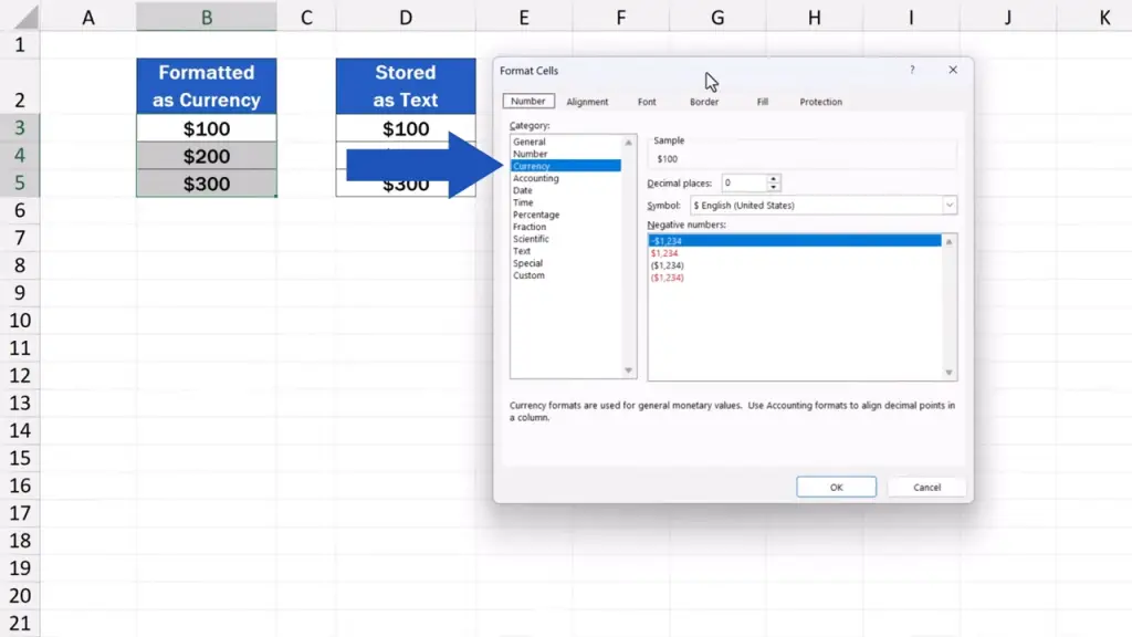
 If we don’t want to use the dollar sign, we need to change formatting. So, in the field ‘Category’ we make a change from ‘Currency’ to ‘Number’.

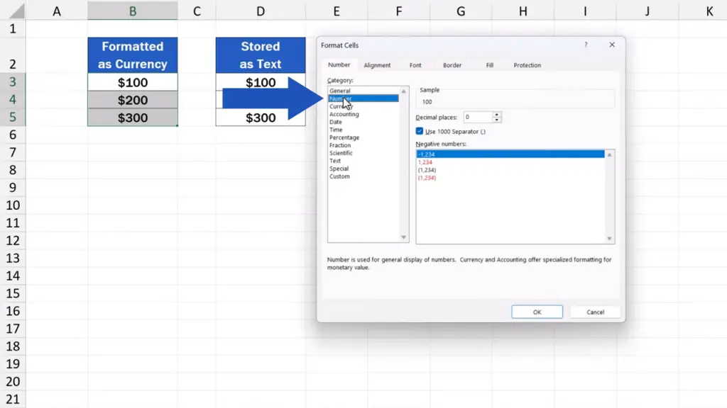
We can make some little adjustments here if needed, like set the number of decimal places or the thousand separator.

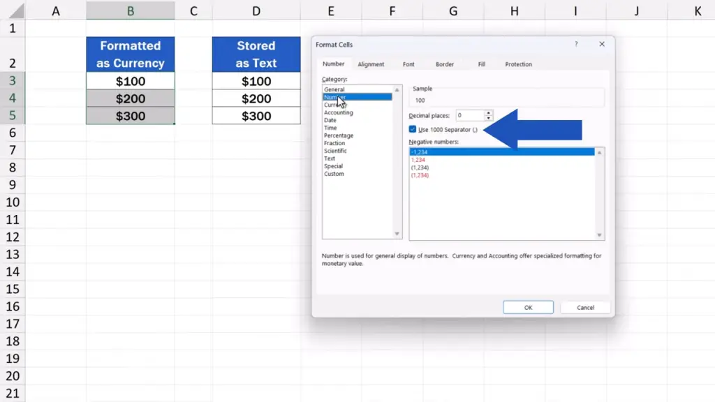
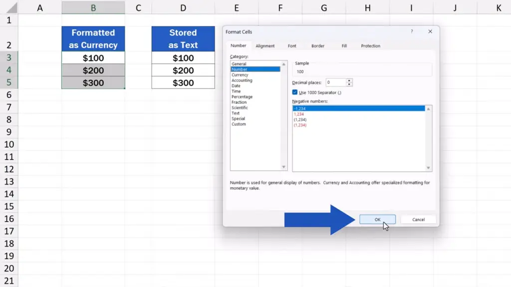
For now, we simply leave these extra settings the way we found them, press ‘OK’, and that’s it!

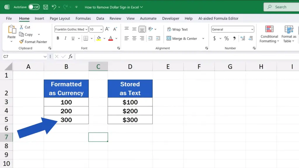
The dollar sign has disappeared from all three cells, but the numbers haven’t changed.

How to remove the dollar sign when it’s part of text

And let’s move on to the next scenario.

In column D, the dollar sign has been manually entered next to the numbers.

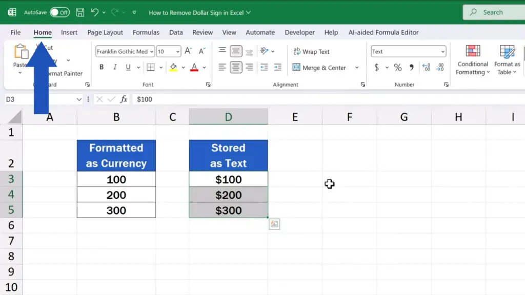
The symbol can easily be removed from all cells at once thanks to a handy little function called ‘Find & Replace’. Again, we select these three cells.

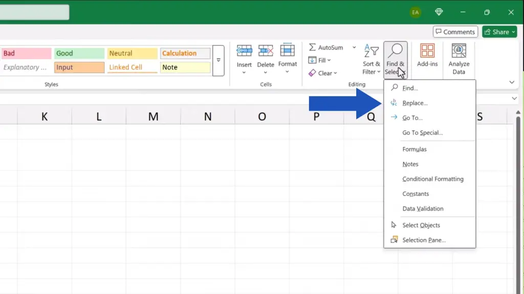
Then we go to the ‘Home’ tab.

Click on ‘Find & Select’.

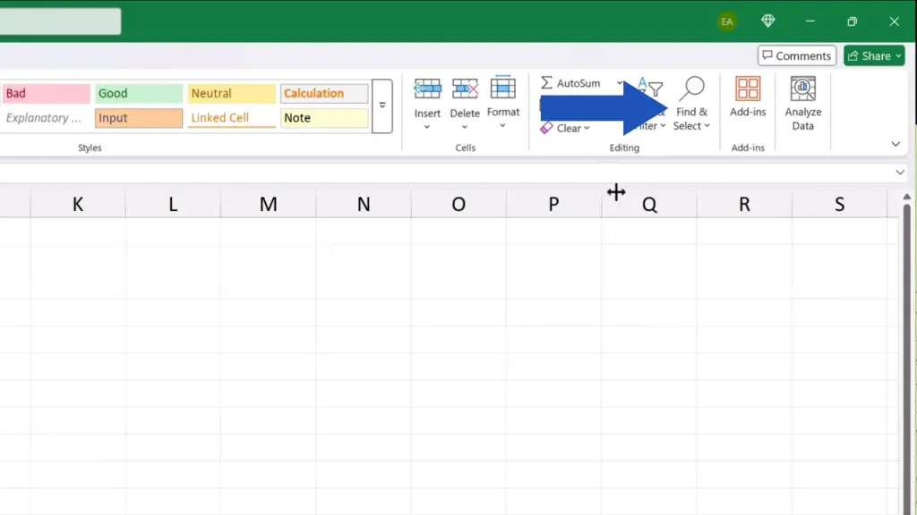
And then click on ‘Replace’ for the ‘Find & Replace’ window to appear.

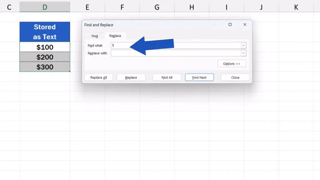
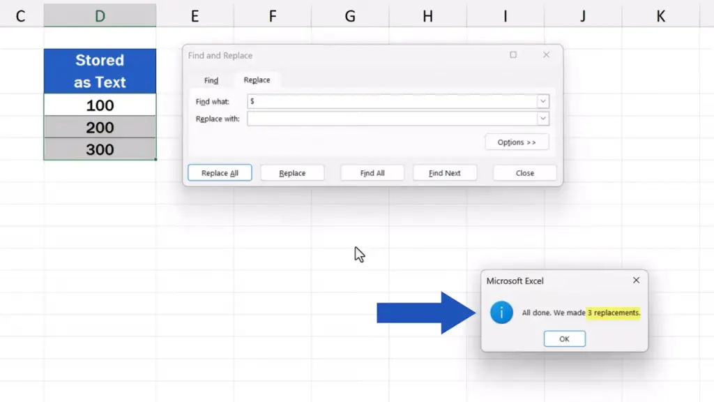
In the field ’Find what’, we type the dollar sign.

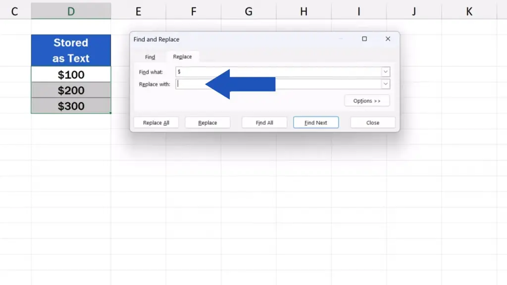
The box ‘Replace with’ remains empty, since we want to find all occurrences of the dollar sign in the selected range of cells and remove them without any replacement.

Now we just simply click on ‘Replace All’ and it’s all done.

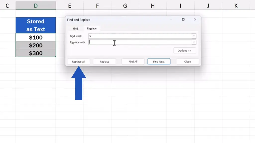
We’re also provided with the information on how many changes have been made. In this case it’s three.

We can close the window and check the data tables.

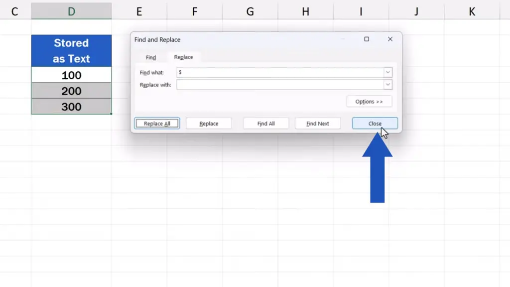
In both cases, the dollar sign has been removed.

Don’t miss out a great opportunity to learn:

• How to Add the Dollar Sign in Excel
• How to Change the Currency in Excel

If you found this tutorial helpful, give us a like and watch other tutorials by EasyClick Academy. Learn how to use Excel in a quick and easy way!

Is this your first time on EasyClick? We’ll be more than happy to welcome you in our online community. Hit that Subscribe button and join the EasyClickers!

Thanks for watching and I’ll see you in the next tutorial!