How to Sort by Color in Excel

Welcome!

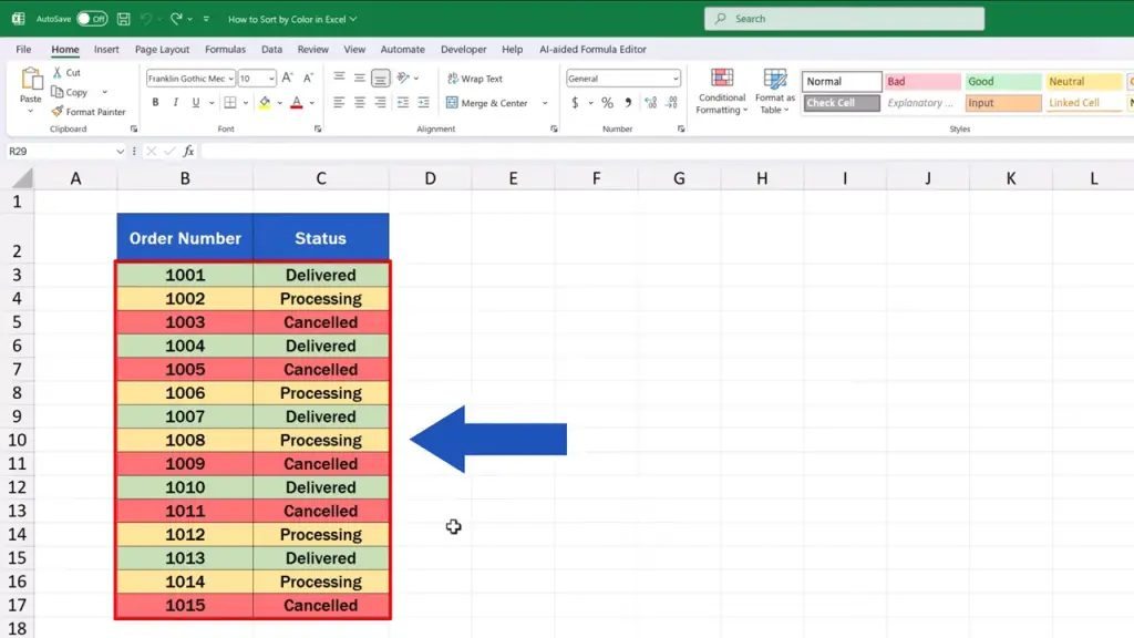
This video tutorial shows how to sort by colour in Excel. Using colours is an excellent way to quickly and conveniently sort data, which can help you towards a clear data overview.

Contents hide

1 How to Open the Sort Dialog to Sort by Colour

2 How to Set a Colour-Based Sorting Condition

3 How to Add Another Level for Colour Sorting

How to Open the Sort Dialog to Sort by Colour

If we want to sort data by colour in Excel, first, we need to click anywhere within the area where the data is stored.

Then we go to the ‘Data’ tab.

And under the section ‘Sort & Filter’.

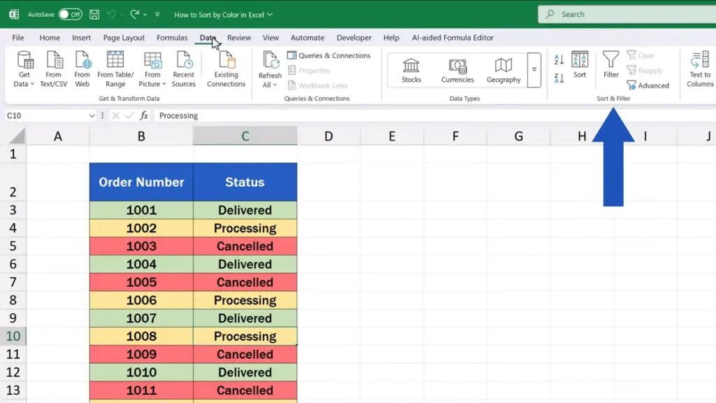
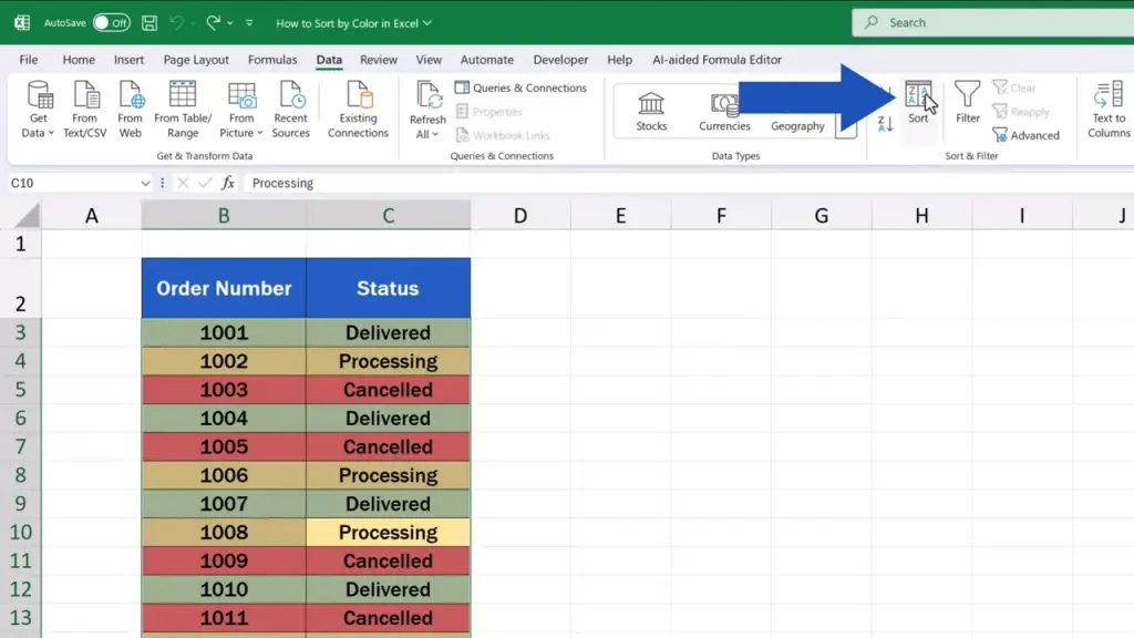
We find the option ‘Sort’.

How to Set a Colour-Based Sorting Condition

When we click on the button, a window appears where we can set how the data will be sorted.

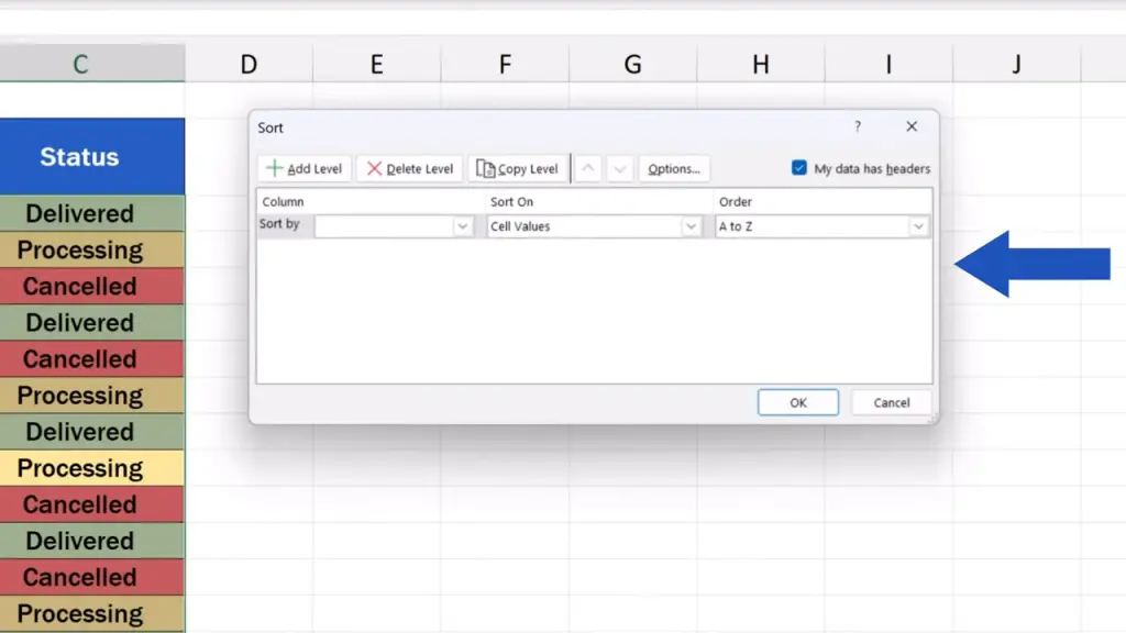
If the data table contains headers, we tick the box ‘My data has headers’ on the right. The first row will then be processed as headers and it won’t be sorted with the rest of the rows.

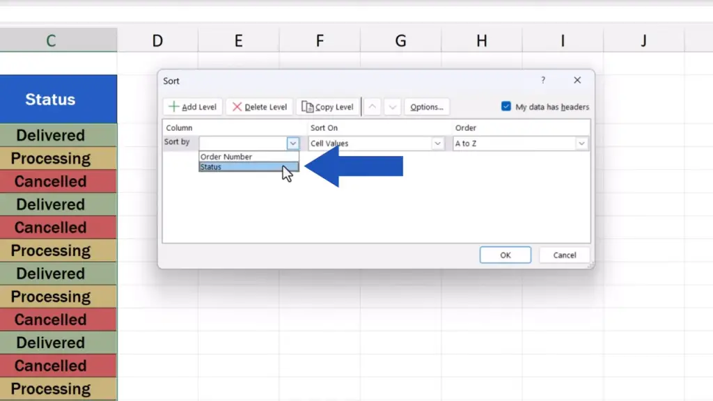
We click on the drop-down menu next to ‘Sort by’ and select the column in which we need the data to be sorted.

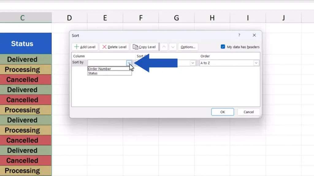
For example, here we’ll go for the column ‘Status’.

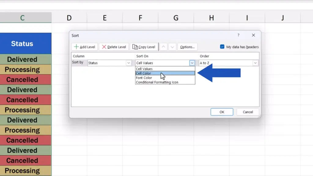
From the next drop-down list marked ‘Sort On’, we choose ‘Cell Color’, because now we want to sort by colour.

If we click on the drop-down menu just below ‘Order’, Excel shows all the colours used in the data table.

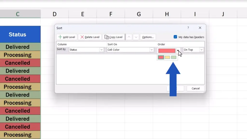
We can choose green first and right next to this field, we can set whether we want to see the green entries at the top or the bottom of the data table.

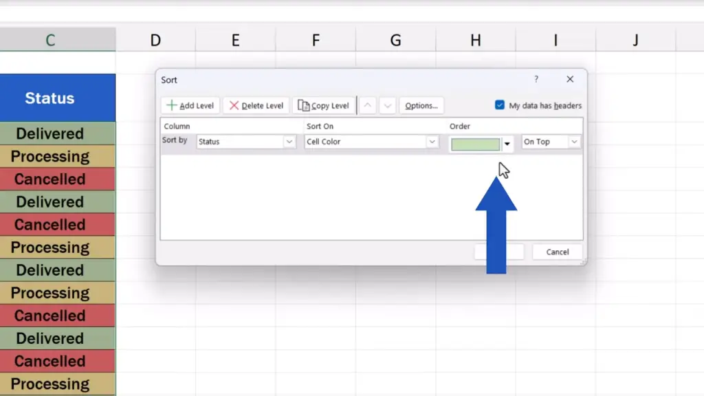
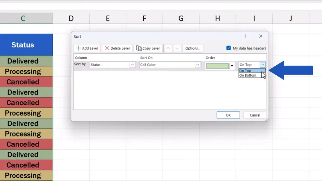
Here, we’ll select ‘On Top’ and we’ll move on.

How to Add Another Level for Colour Sorting

Now, here comes an important thing to remember.

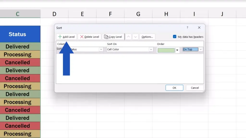
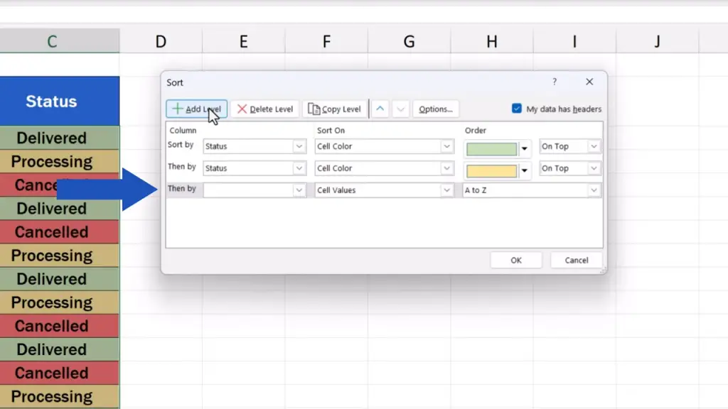
If the data table contains more colours which we want to place in a certain order, we can do so by adding another level.

So, we click now on ‘Add Level’, and we can fill in this new level the same way we did the top one a short while ago.

But now we’ll define the settings for another colour – let’s say yellow.

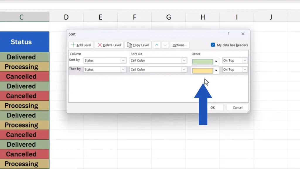
We can place the yellow entries on the top, too. This will cause the green entries to appear above the yellow entries, because the green colour has been set for the first level, whereas the yellow colour shows in the second level.

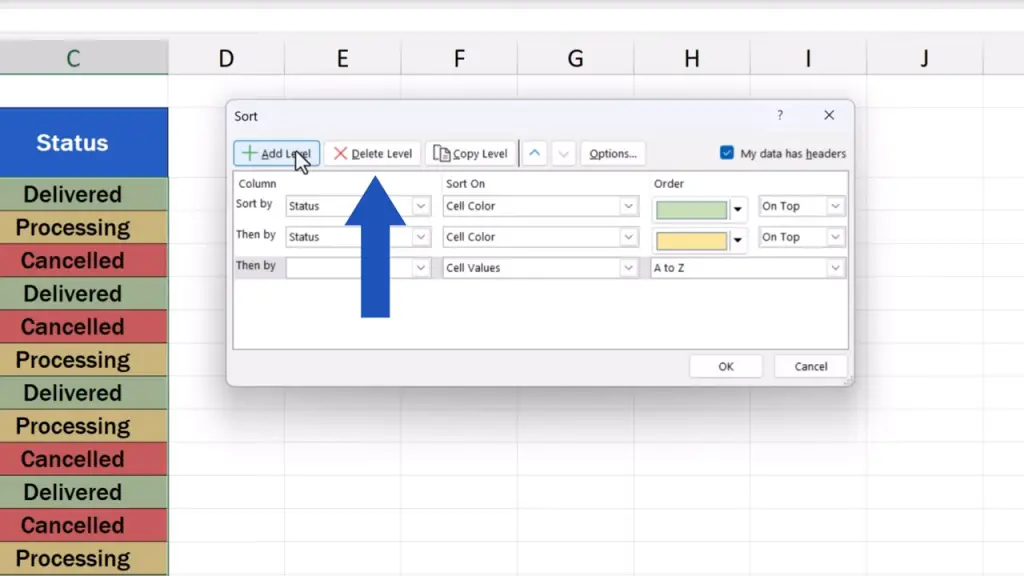
Since there are only three colours in our data table, we don’t need to add a separate level for the red colour. Excel will automatically place the red entries on the very bottom of the data table. But if you really want, you can create an individual level for the third colour, too.

We’re not going to create a third level now, so we can simply remove it using the ‘Delete Level’ button.

Once all has been defined, we’ll just press ‘OK’ and that’s all it takes!

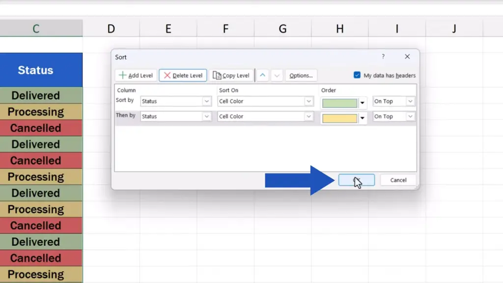
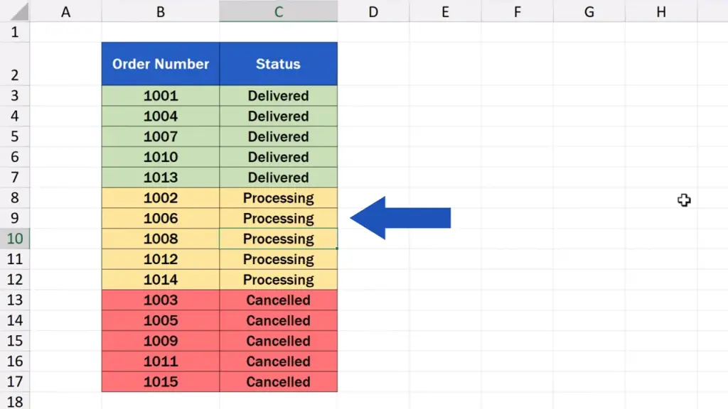
The data table’s been sorted by colour just as we specified – the green entries on the top, the yellow ones right below, and the red rows come at the very bottom of the data table.

This is a simple way to sort any data by colour in a data table of any size. Try it out and make sure to let us know how it went in the comments section below. We’ll be thrilled to hear from you!

Don’t miss out a great opportunity to learn:

If you found this tutorial helpful, give us a like and watch other tutorials by EasyClick Academy. Learn how to use Excel in a quick and easy way!

Is this your first time on EasyClick? We’ll be more than happy to welcome you in our online community. Hit that Subscribe button and join the EasyClickers!

Thanks for watching and I’ll see you in the next tutorial!

Don’t miss out a great opportunity to learn:

If you found this tutorial helpful, give us a like and watch other tutorials by EasyClick Academy. Learn how to use Excel in a quick and easy way!

Is this your first time on EasyClick? We’ll be more than happy to welcome you in our online community. Hit that Subscribe button and join the EasyClickers!

Thanks for watching and I’ll see you in the next tutorial!