How to Add a Slicer in Excel
Welcome!
In this tutorial, we’ll be talking about how to add a slicer in Excel in a quick and easy way. Slicers provide an interactive way to filter data and obtain the information you need promptly.
Let’s see how it’s done then!
How to Insert a Slicer in a Table
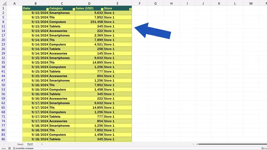
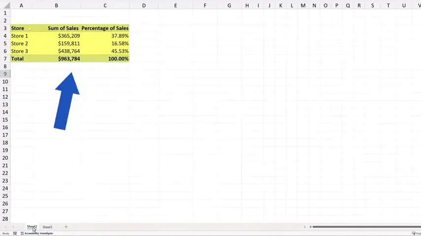
To start with, I’d like to mention that we can use the slicer in Excel most conveniently when the data are formatted as a table or if a pivot table’s been created, which of course we’ve done here, in the other sheet.
Today, we’re going to focus only on how to add a slicer.
And let’s start with the first case, which is the situation where the data’s been formatted as a table.
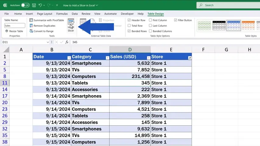
To insert a slicer, click anywhere within the table area.
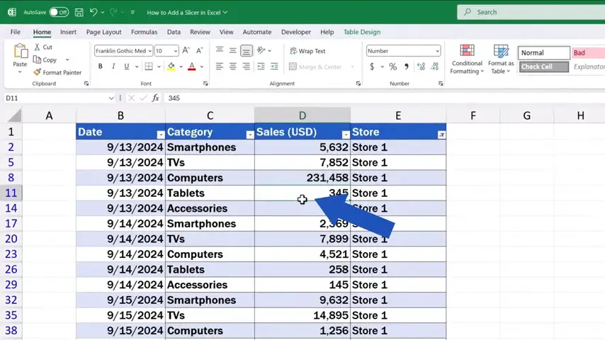
And find the ‘Table Design’ tab up here.
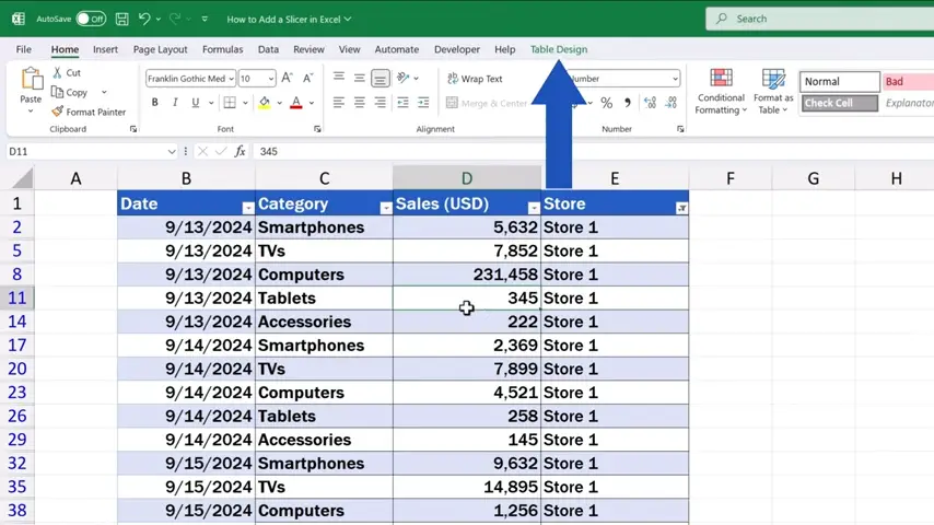
Go to the tab and click on ‘Insert Slicer’.
A window pops up where we can pick items based on which we’ll be able to filter the data.
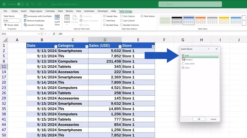
For instance, we can select ‘Store’, ‘Category’, and ‘Date’. After we confirm with ‘OK’.
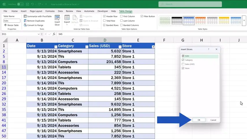
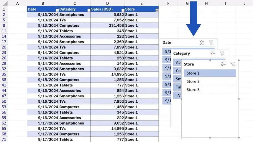
Excel inserts all three selected slicers in the sheet.
How to Insert a Slicer in a Pivot Table
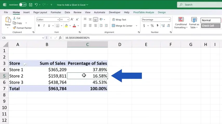
We can also insert a slicer when working with a pivot table in a simple way. Let’s click into Sheet2 now where we can see the prepared pivot table.
So, we’re going to go through how to insert a slicer for the pivot table and then we’re going to have a closer look at how we can work with and modify each slicer according to what we need.
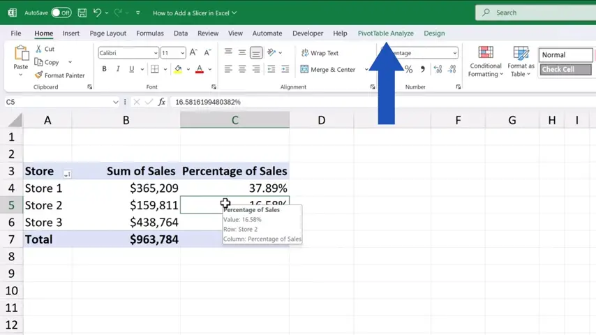
To insert a slicer, click anywhere within the pivot table.
Then go to the ‘PivotTable Analyze’ tab where we can find ‘Insert Slicer’.
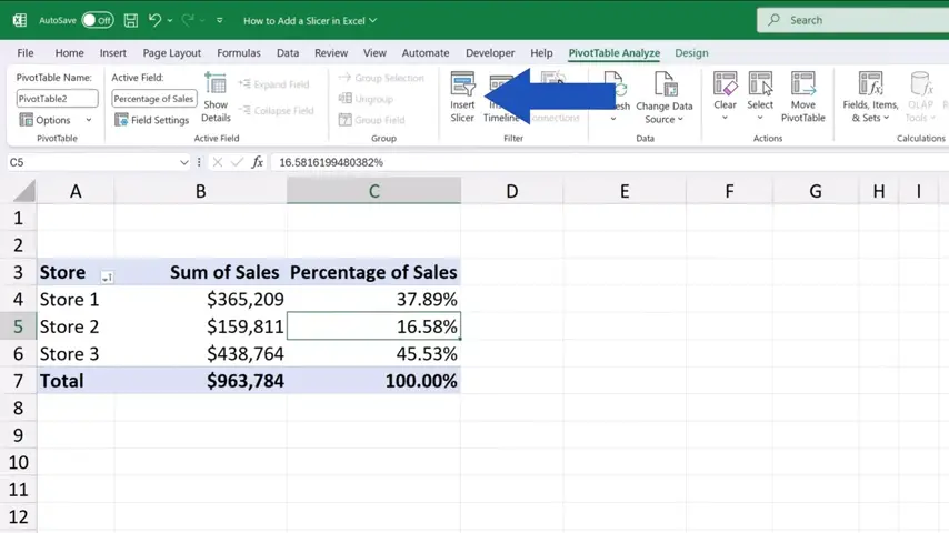
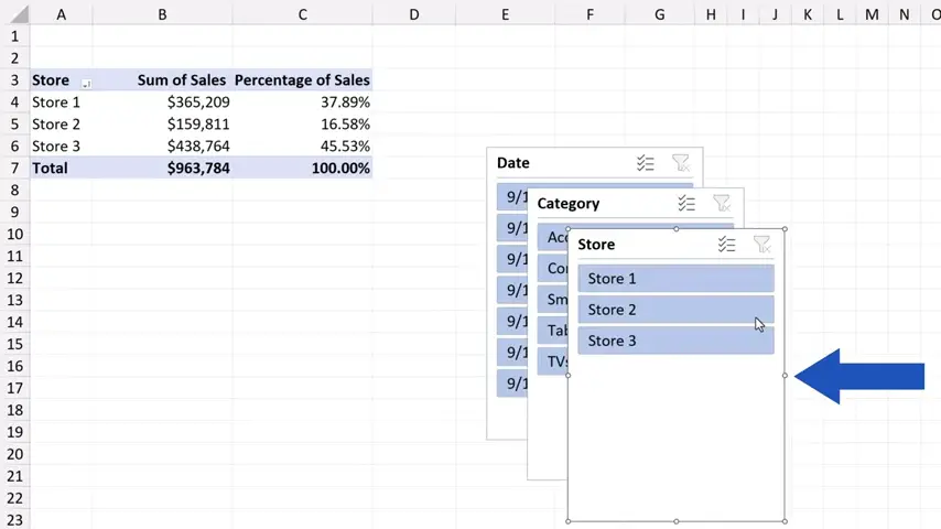
We click on it and here we select for example ‘Store’, ‘Category’ and ‘Date’ again.
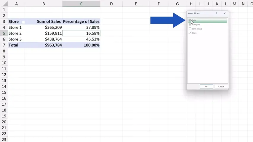
And again, after hitting ‘OK’, the slicers appear on the screen right away.
Well, that would be it regarding how to insert a slicer and we can move on now to the latter part!
How to Modify and Move Slicers
Together we’ll see how we can modify and adjust each slicer based on what we need. You’ll be able to use all the little tricks for all slicers, whether you’ve formatted the data as a table or simply created a pivot table.
Since we’re already working with the pivot table, we can take a look at how to do all that here.
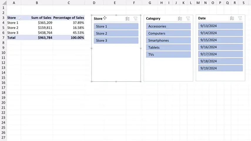
Each slicer can be moved around and set anywhere within the sheet. Simply, click on the slicer header and drag and drop it wherever needed. Here, for example, we arrange the slicers in this order.
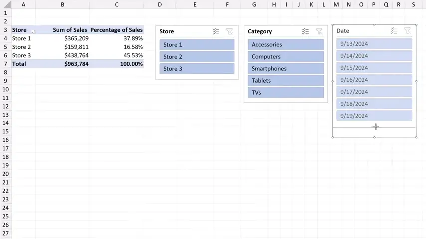
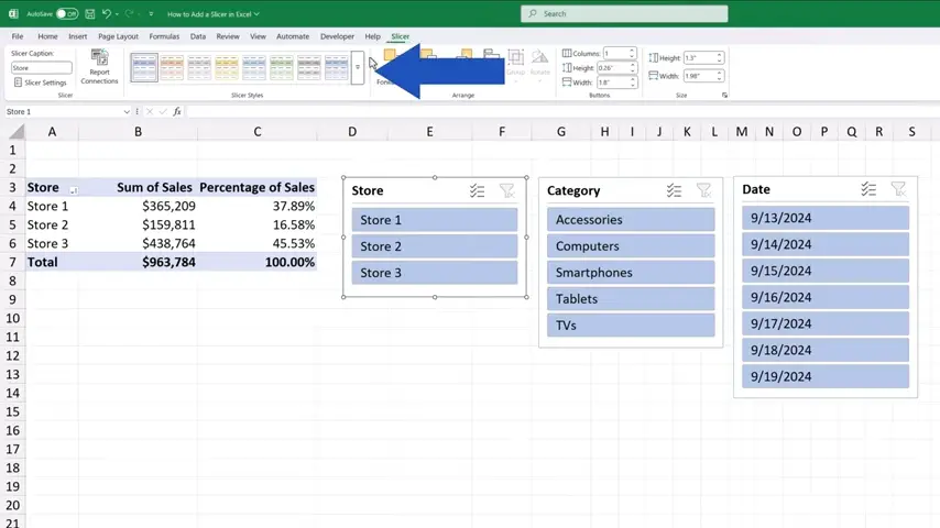
Now we can use these points, these little circles, to change the size of the slicer.
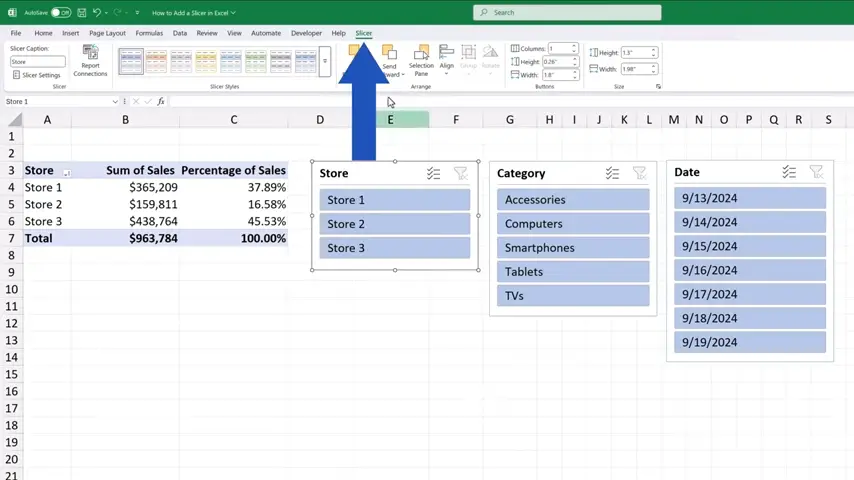
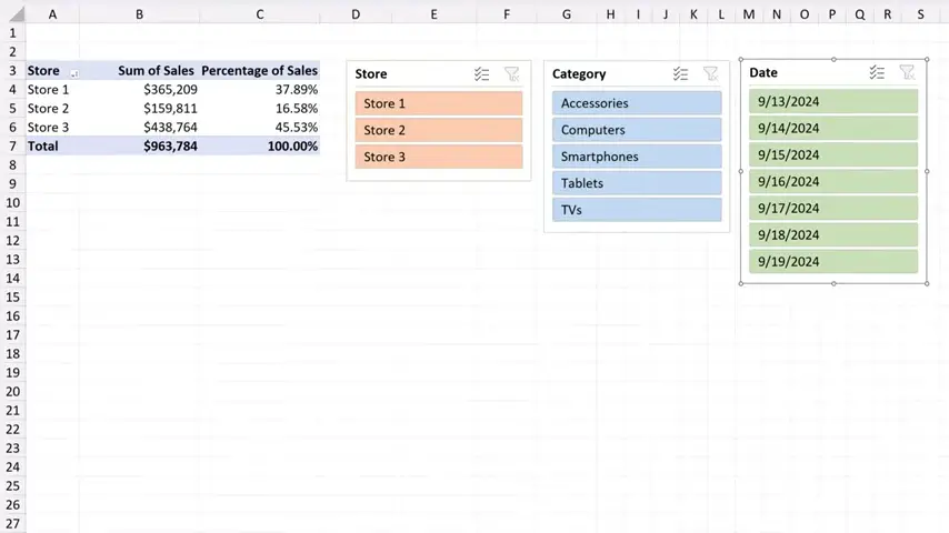
To make everything clear and visible, and for easier navigation through the data, we can use a different colour for each slicer. Let’s say we use orange for this slicer, blue for that one, and the third slicer will be green.
How to Filter Data Using Slicers
We can move on and have a look at how to use slicers to filter data.
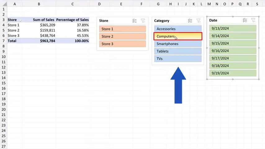
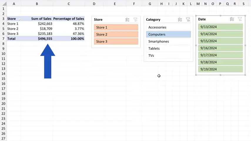
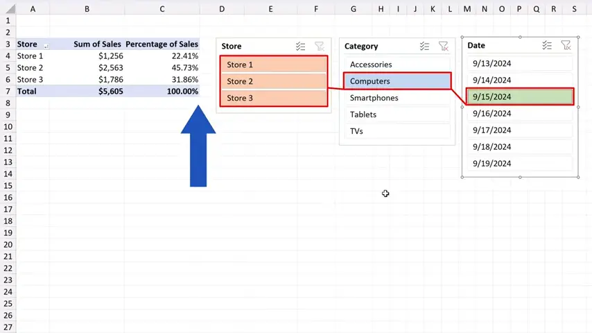
To filter the Computers sales data, we simply click on ‘Computers’ in the slicer ‘Category’. We can immediately see the sales figures in ‘Computers’ for all three stores.
To filter the sales for a particular day, we can click on a specific date in the ‘Date’ slicer. Let’s select the 15th September 2024.
And here we come with the Computers sales for the 15th September 2024.
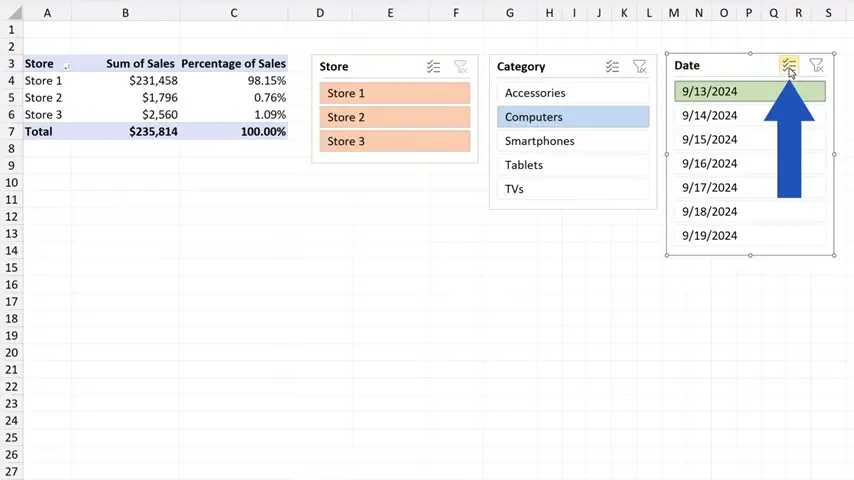
But there’s one thing to be aware of here.
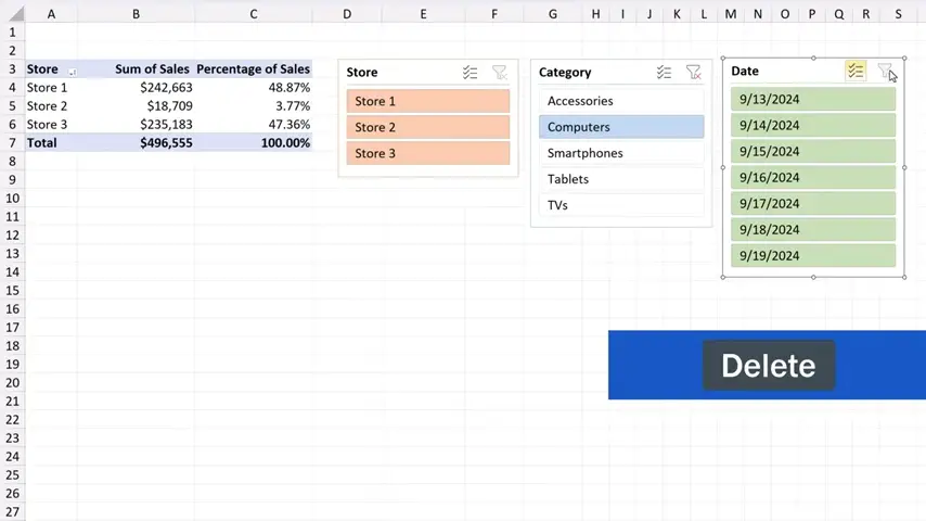
Excel normally allows you to select only one option per slicer. To see data for more than one day, we need to click on the ‘Multi-Select’ button up here.
Then we can go ahead and choose more than one date, so we can go for the 13th, 14th and the 15th now.
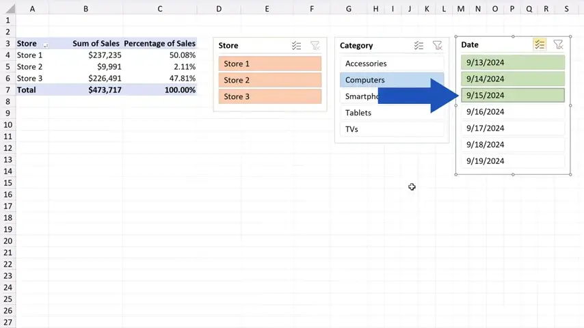
Great! The sales for these three days now show in the table.
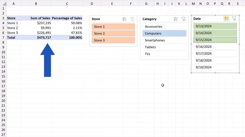
Slicers are an amazing tool if we want to organise and display data in a table in a neat and interactive way, and according to what we need.
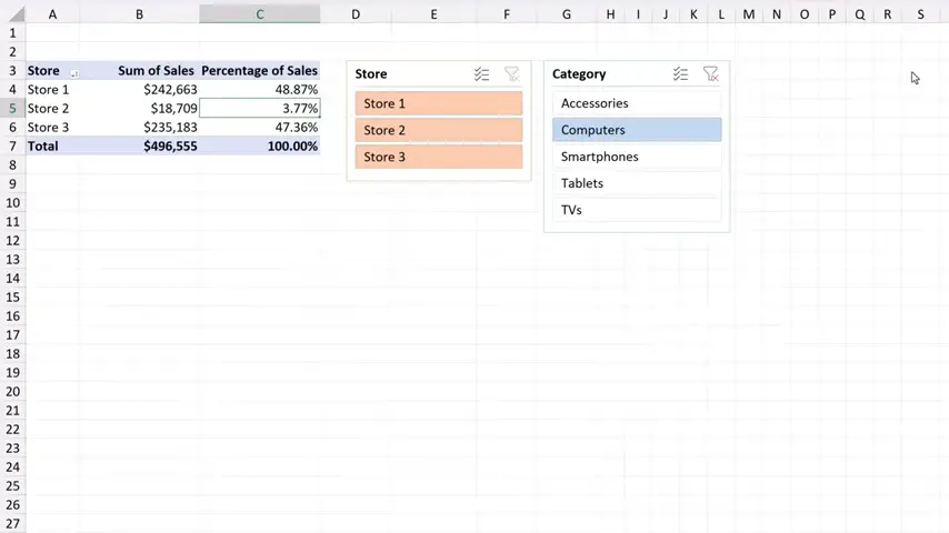
And if we don’t need a slicer, we can simply click on it and clear the filter using this button, which basically makes all data in the table available again.
Then we simply hit ‘Delete’ on the keyboard and that’s it – the slicer’s gone!
Don’t miss out a great opportunity to learn:
If you found this tutorial helpful, give us a like and watch other tutorials by EasyClick Academy. Learn how to use Excel in a quick and easy way!
Is this your first time on EasyClick? We’ll be more than happy to welcome you in our online community. Hit that Subscribe button and join the EasyClickers!
Thanks for watching and I’ll see you in the next tutorial!

 How to Subtract a Percentage in Excel
Welcome! Today we’re going to talk about the simplest way how to…


