How to Make a Table in Excel (Format as Table)

In this tutorial, we’re going to have a look at how to make a table in Excel. Thanks to the function ‘Format as Table’, data can be neatly organised and visually represented in a clear formatted table. Moreover, various powerful features are available for use in such data tables.

So, let’s have a look at all that!

How to Create a Table in Excel

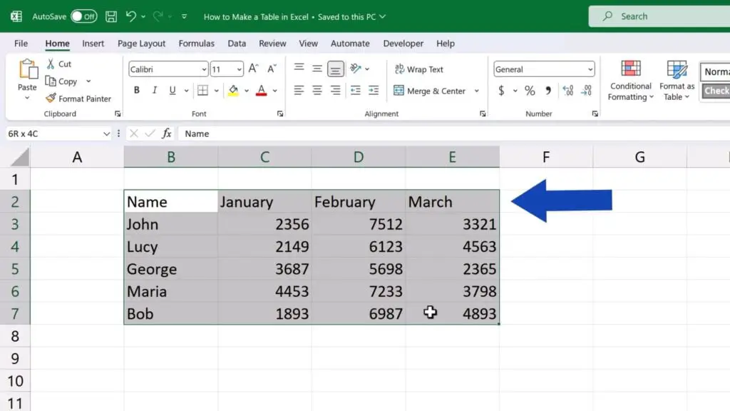
To make data look clear and well-organised, creating a table is a great idea. So, first we need to select all the data we want to put in a table.

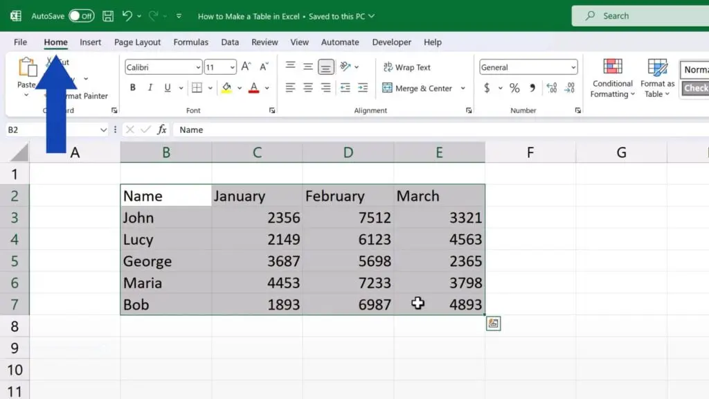
Then we click on the ‘Home’ tab and in the section ‘Style’, we click on ‘Format as Table’.

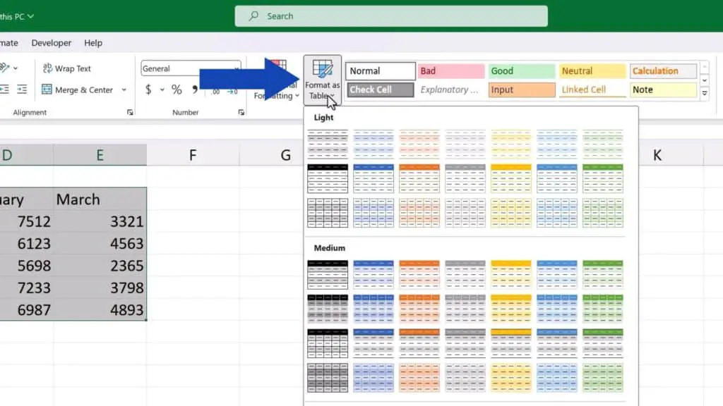
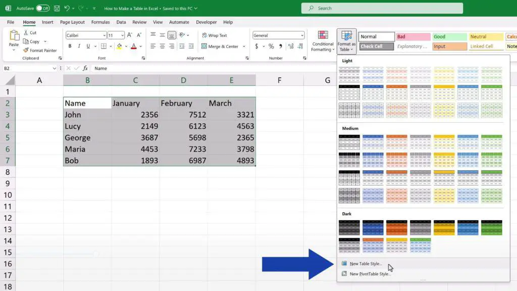
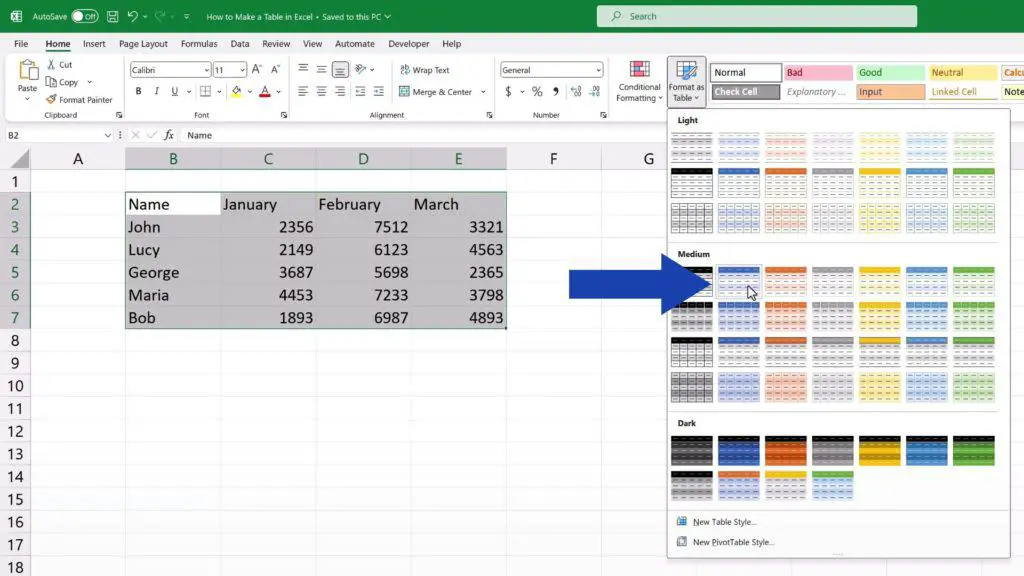
Now we see all the available styles Excel offers. We can choose a colour we like or we can create our own style by clicking on the button down here.

We’ll go for one of the predefined styles now, the blue one.

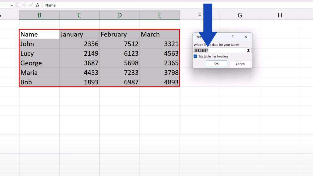
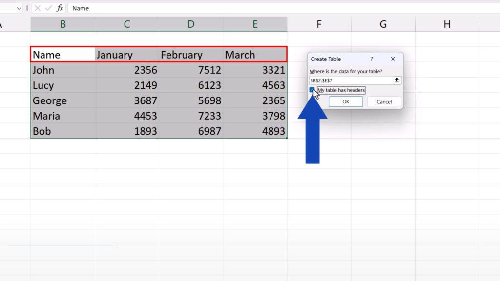
So, let’s click on it and another window appears where we can specify two things – our data range, which we have already defined by selecting it at the beginning and there’s a question whether the data table has a header, which our table does, so we make sure this tick box is selected.

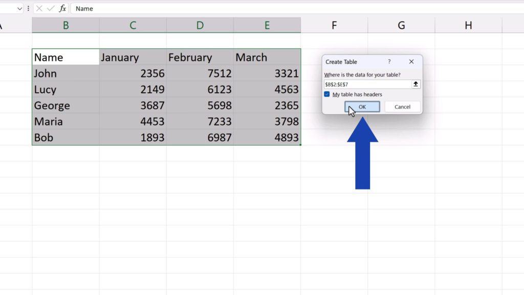
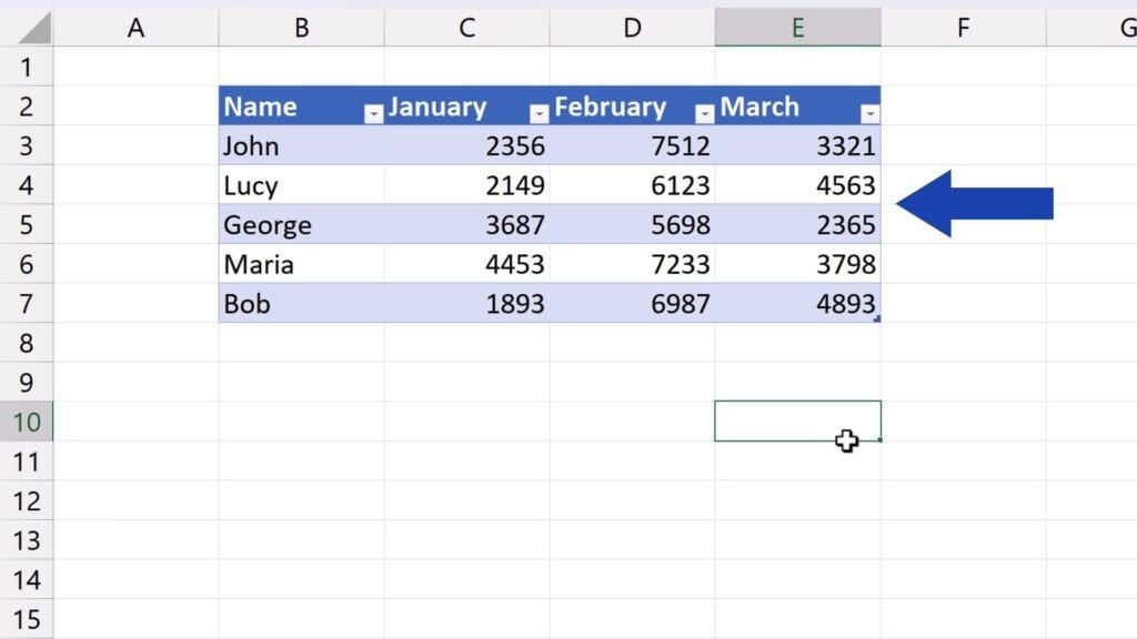
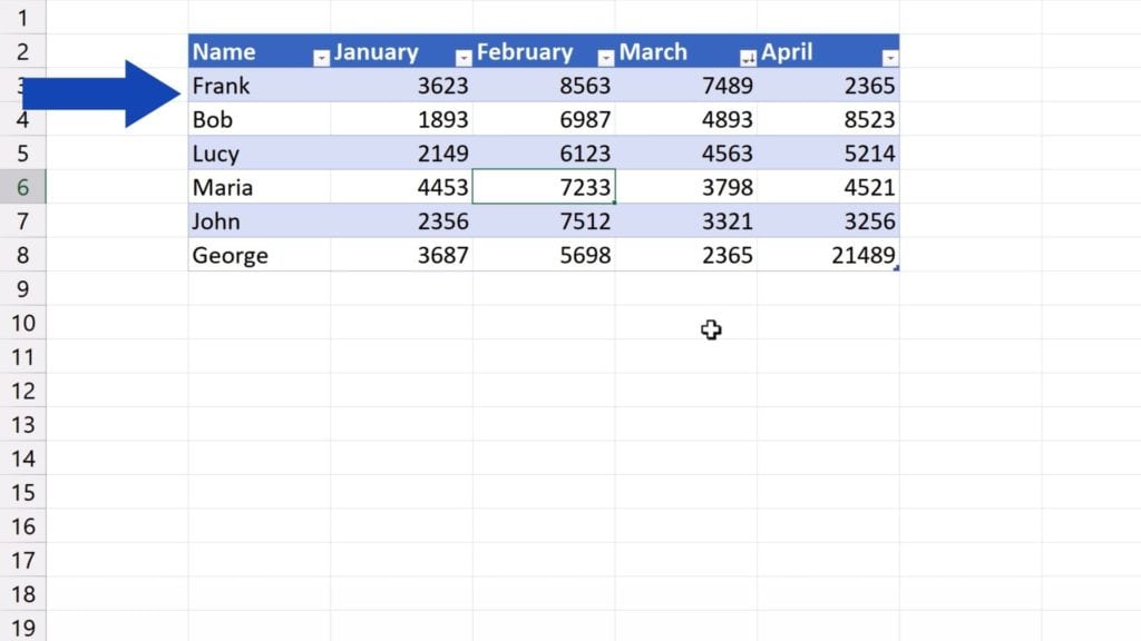
As soon as we hit OK, the data table shows in the style we’ve chosen.

How to Add Something In a Formatted Data Table

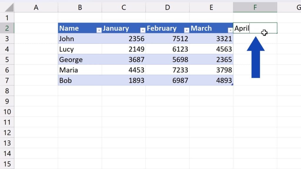
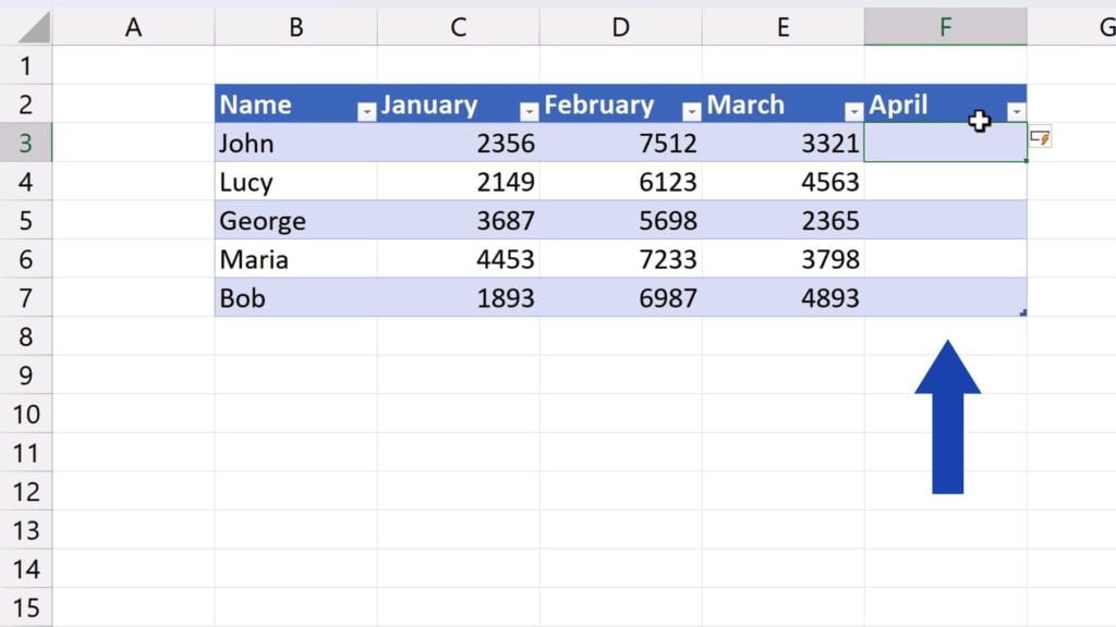
If you decide to add something in a formatted data table, that’s no problem at all. Let’s say we want to add data for April, so we type ‘April’ in the column F and press Enter. And here we go! The data table’s been expanded and we can comfortably add the data for April.

How to Add a Row In a Formatted Data Table

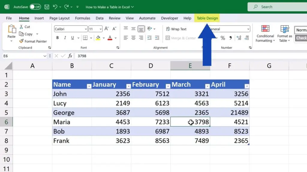
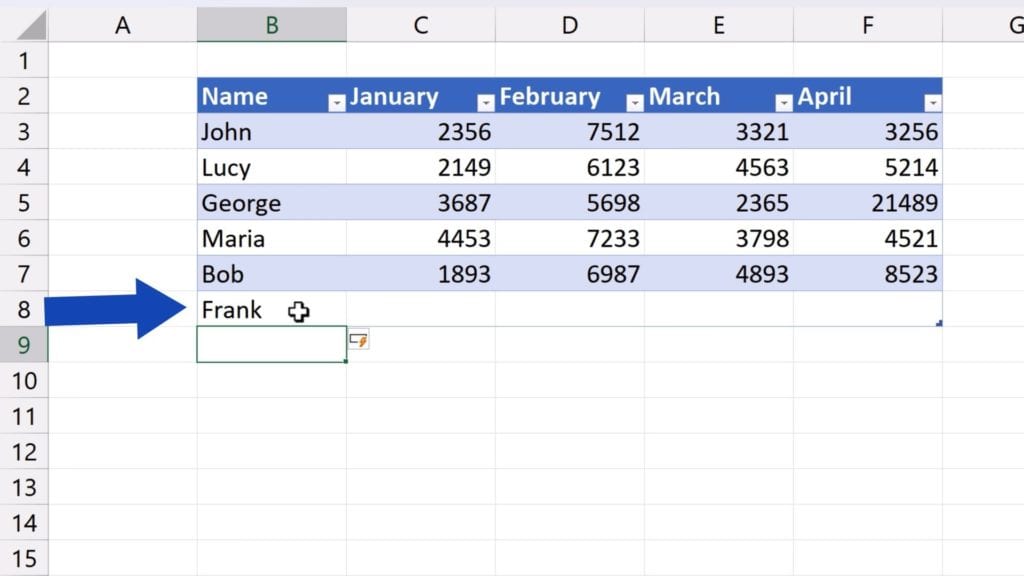
The same works with rows. So, if we need to add a row, we just type let’s say ‘Frank’ in B8, press Enter and that’s all it takes. Now we can add Frank’s data into the table with the formatting being automatically applied to the new row, too.

Now, there’s one important thing worth noting.

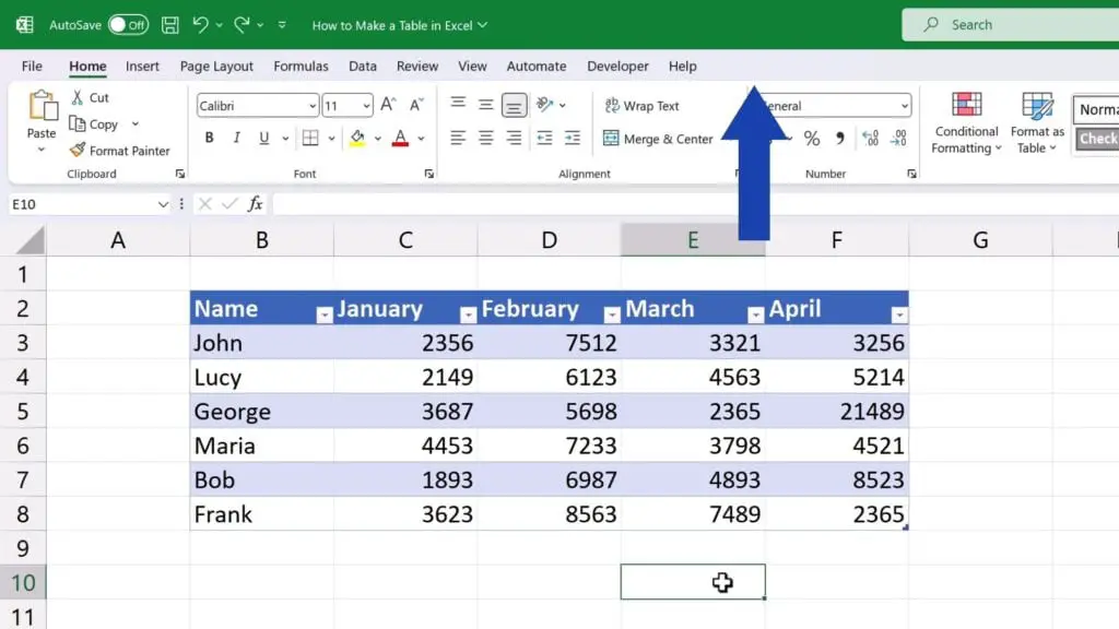
Thanks to the function ‘Format as Table’ we’ve just used, Excel opens a new tab on the Ribbon, which says ‘Table Design’. It’s available only when you click into the table. If you click outside the table borders, the tab will disappear.

Let’s click into the table again and have a look at what we can do in our data table thanks to this new ‘Table Design’ tab.

How to Use ‘Table Design’ Tab

First, we’ll go through the option of changing colour styles. Simply, click on this button on the right in ‘Table Styles’ and pick whichever style you want.

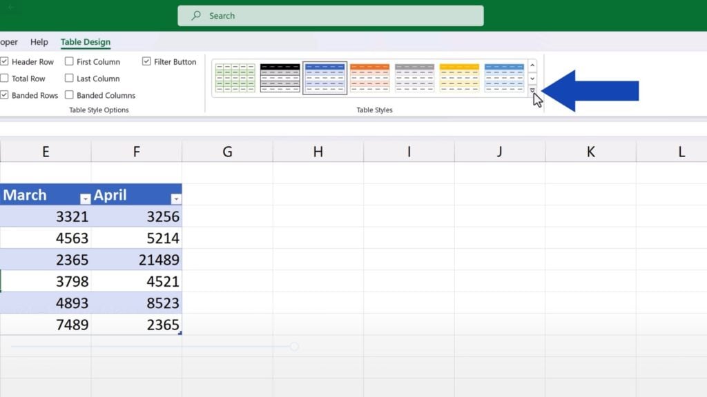
We can now try the green one and switch back to the blue one again.

Let’s move on and have a look at various powerful features available in the formatted table.

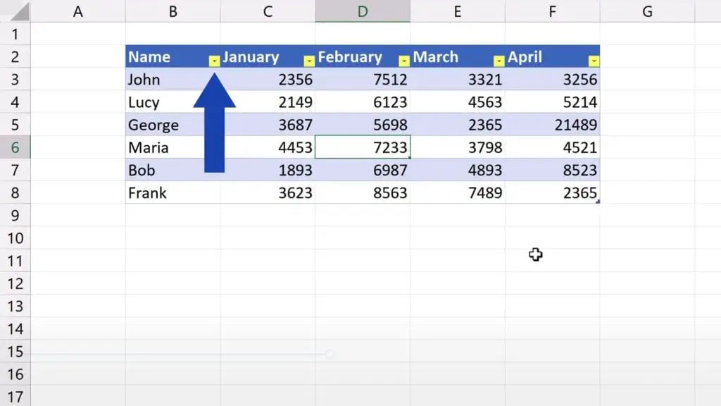
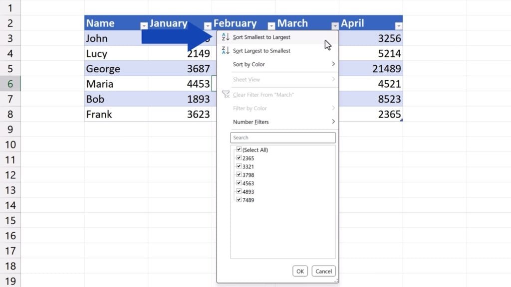
You’ve most probably noticed these drop-down buttons in the header. Thanks to them you can conveniently sort the data in the table. For example, we can sort the March values from smallest to largest or vice versa.

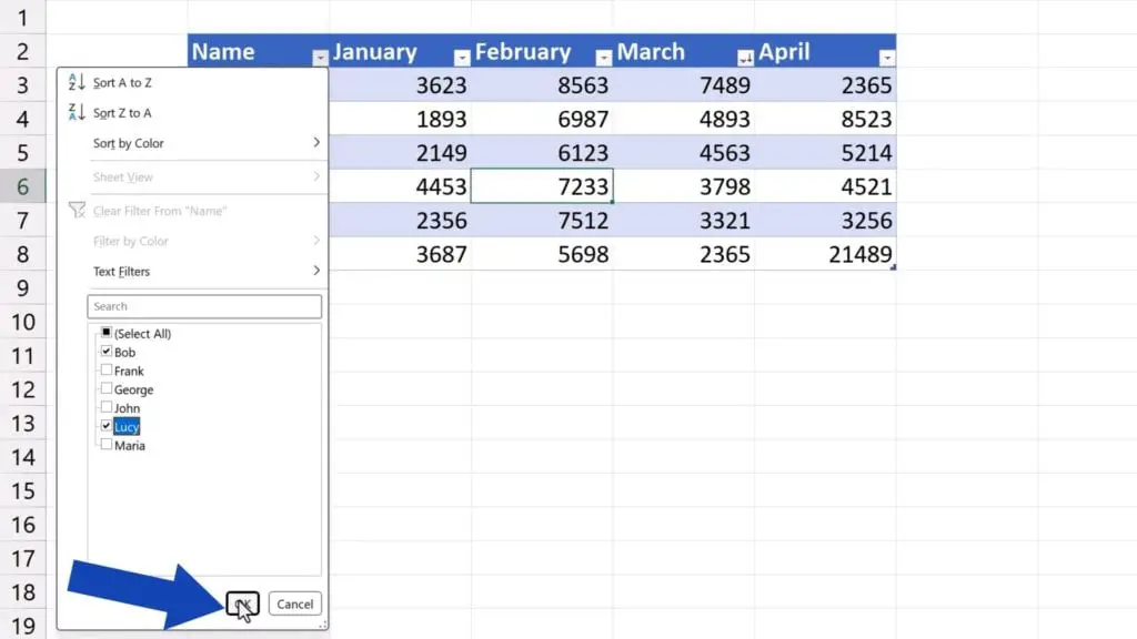
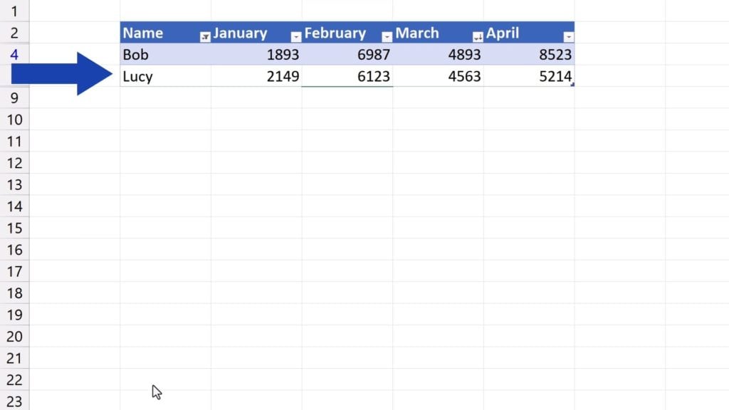
We can also filter data out, for instance if we want to see only the data for Bob and Lucy. So, we’ll click on the button in the column ‘Name’, here we’ll untick ‘Select All’ and we’ll put a tick next to Bob and Lucy. We press OK and here they are! If we want to see all the data again, we’ll click on the Filter button one more time and click on ‘Clear Filter From “Name”’.

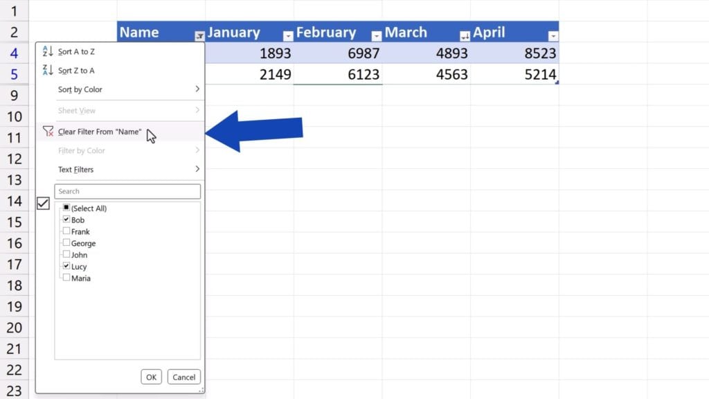
All the data appear in the table again.

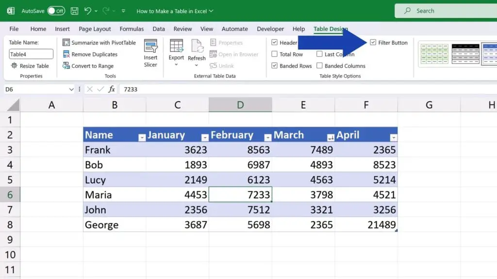
You can disable the Filter buttons in a table or enable them again any time. To show the Filter buttons, you need to keep the option ‘Filter Button’ up here selected. If you unselect the box, the buttons will disappear.

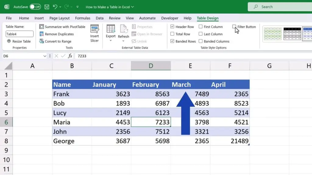
We can disable the buttons at the moment and move on to see other features of a formatted table.

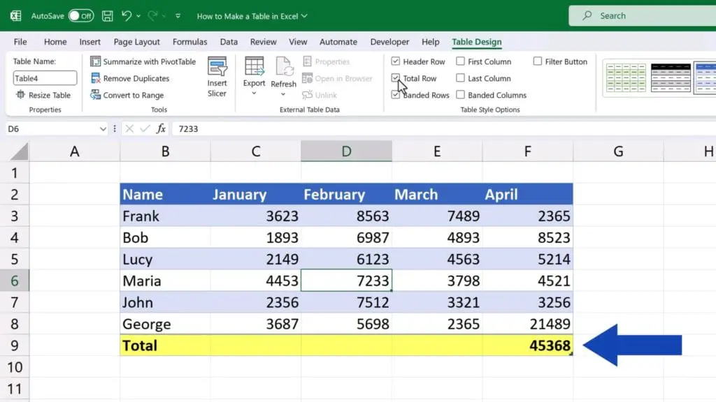
Another super powerful feature, which is also super useful, is ‘Total Row’. If we tick the box, a row will be added at the end of the table to show the total for a column.

If we click on the cell, there’s a drop-down button which offers other functions, so we can choose from ‘Average’, ‘Count’ values, ‘Maximum’ value or ‘Minimum’ value, and many others.

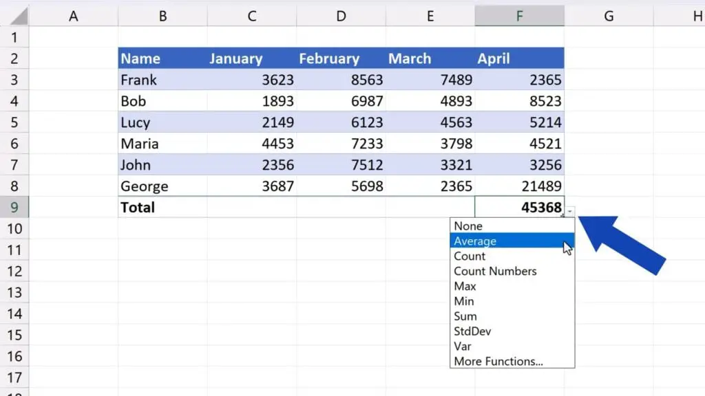
You can choose any function for any column according to what you need. So, let’s say we’ll go for ‘Average’ here, here we’ll put ‘Count’ and here, for example, ‘Max’.

Or we can simply copy one function to the rest of the columns through dragging the bottom right-hand corner of the cell containing the function.

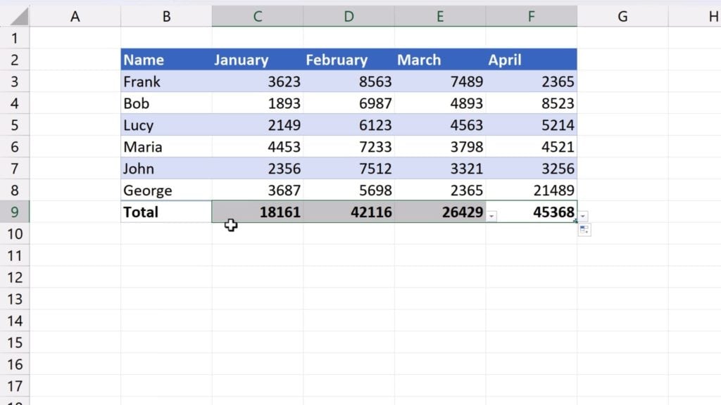
And that’s it. The Total row now shows the sum in all columns of our data table.

If you don’t need to show the calculations in the last row, simply untick the option ‘Total Row’ and everything will disappear right away.

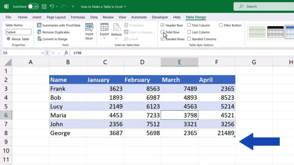
Let’s move on and have a look at more features in the section ‘Table Style Options’, now.

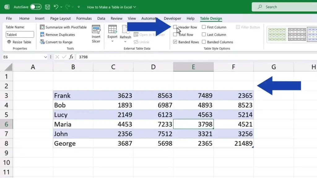
The option ‘Header Row’ turns on or off the header.

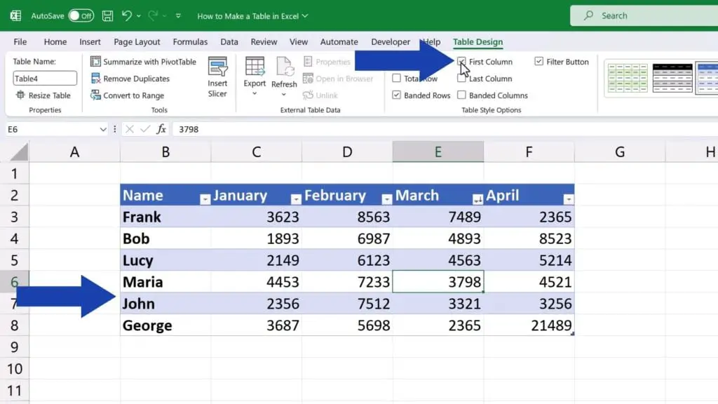
‘First column’ will highlight the data in the first column in bold.

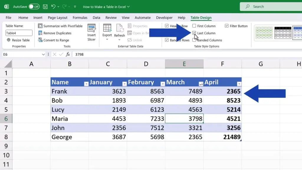
‘Last Column’ does the same, but in the last column of the data table instead of the first one.

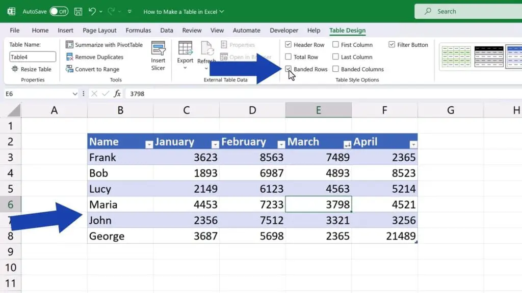
The option ‘Banded Rows’ highlights every other row in the table for better orientation.

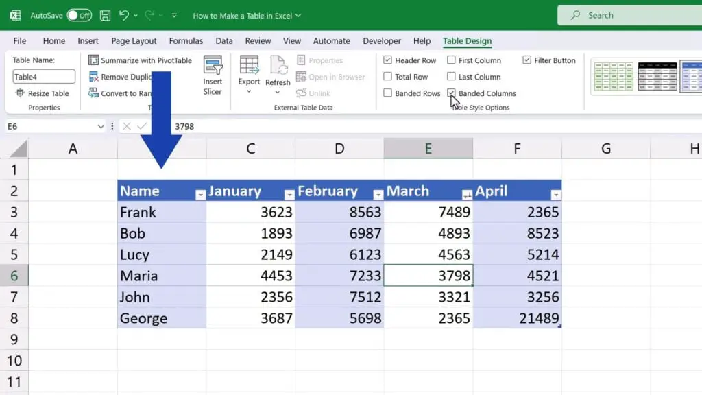
‘Banded Columns’, on the other hand, highlights every other column.

Of course, ‘Table Design’ tab offers other, more advanced features which can be a great help when working with data in a table. But in this tutorial, we wanted to go mainly through the basic ones. If you’d like to see some of the advanced features, leave us a note in the comments section and we’ll be happy to prepare a video tutorial for any other feature available when working with ‘Format as Table’ function.

To wrap it up, we’ve got a tip for another video by EasyClick Academy worth watching – a detailed tutorial on how to remove table formatting in Excel. You’ll see three different levels on which we can remove table formatting. That’s why we’re offering a separate tutorial, the link to which you can find in the list below.

Don’t miss out a great opportunity to learn:

• How to Remove Table Formatting in Excel
• How to Use Color Scales in Excel (Conditional Formatting)
• How to Clear Formatting in Excel (The Simplest Way)

If you found this tutorial helpful, give us a like and watch other tutorials by EasyClick Academy. Learn how to use Excel in a quick and easy way!

Is this your first time on EasyClick? We’ll be more than happy to welcome you in our online community. Hit that Subscribe button and join the EasyClickers!

Thanks for watching and I’ll see you in the next tutorial!