How to Add Data Validation in Excel

In this video tutorial, we’ll have a look at how to add Data Validation in Excel in a quick and easy way. Through this useful feature, we can set what data can and what can’t be entered into a cell with the result being exact, reliable and consistent data tables.

Contents hide

1 How to Set General Data Validation Rules

2 How to Set Up an Input Message in Excel

3 How to Set Up an Error Message for Invalid Data

4 How to Remove Data Validation

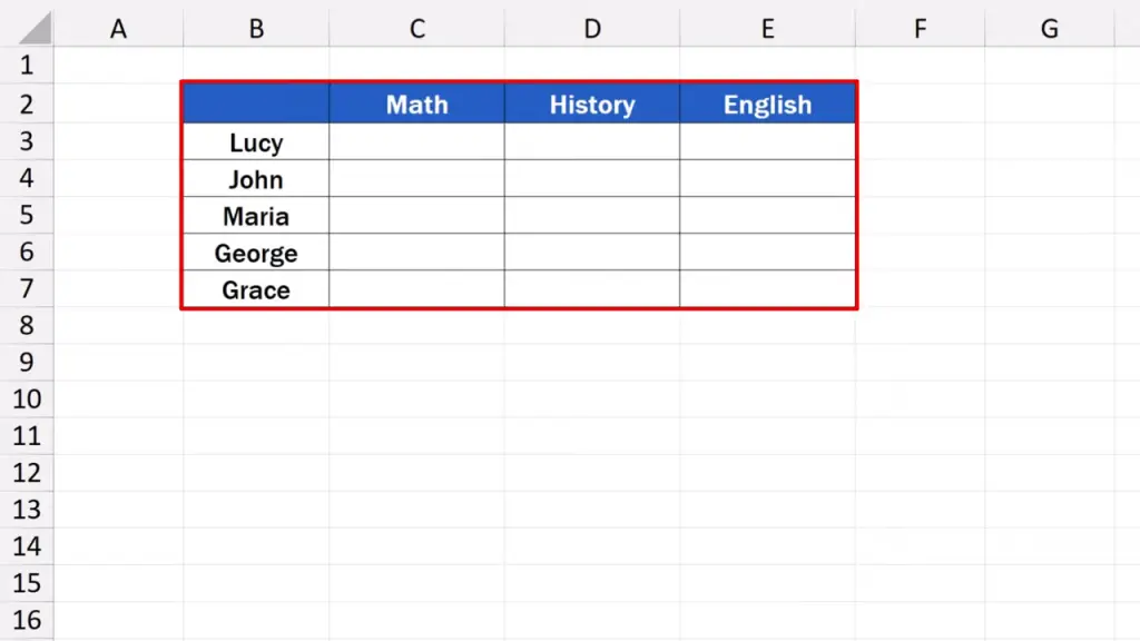
We’re going to use this simple example to explore Data Validation in Excel. Here’s a data table with five students and three subjects. Let’s say these students will be tested and each student can get a score of 0 to 100 in each subject. These results will be entered into the data table by various teachers.

And here comes the feature Data Validation! Thanks to Data Validation, we can adjust the settings of each cell, so anyone working with the table can type in just a number from 0 to 100 and nothing else.

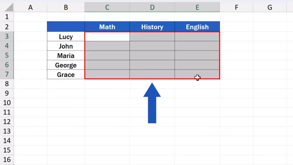
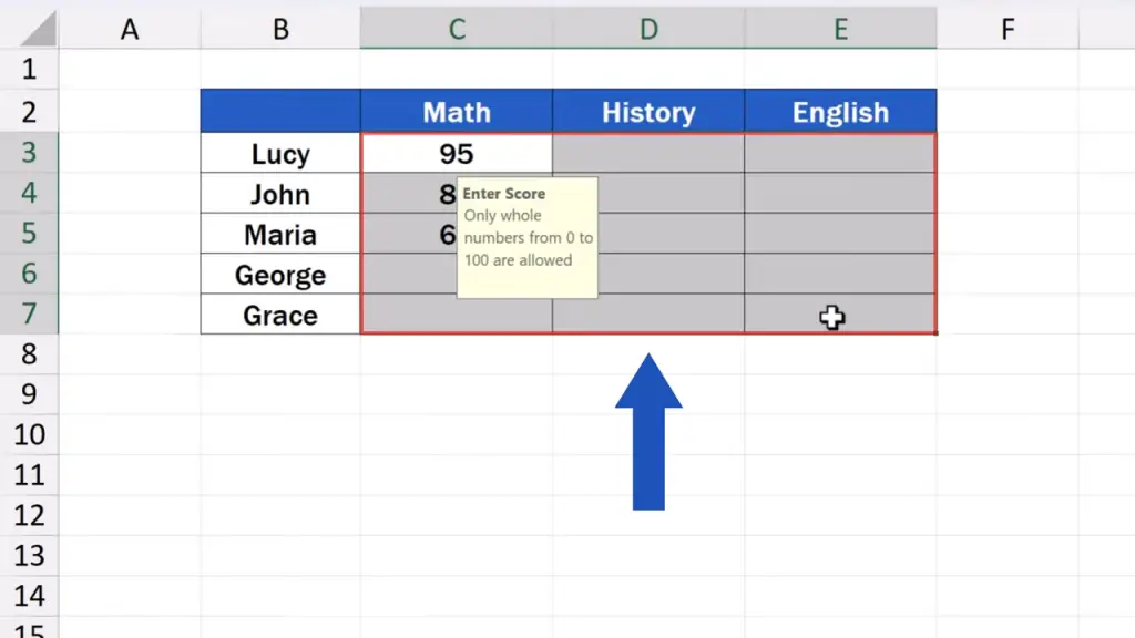
First, we select the area where we want the Data Validation settings to apply.

How to Set General Data Validation Rules

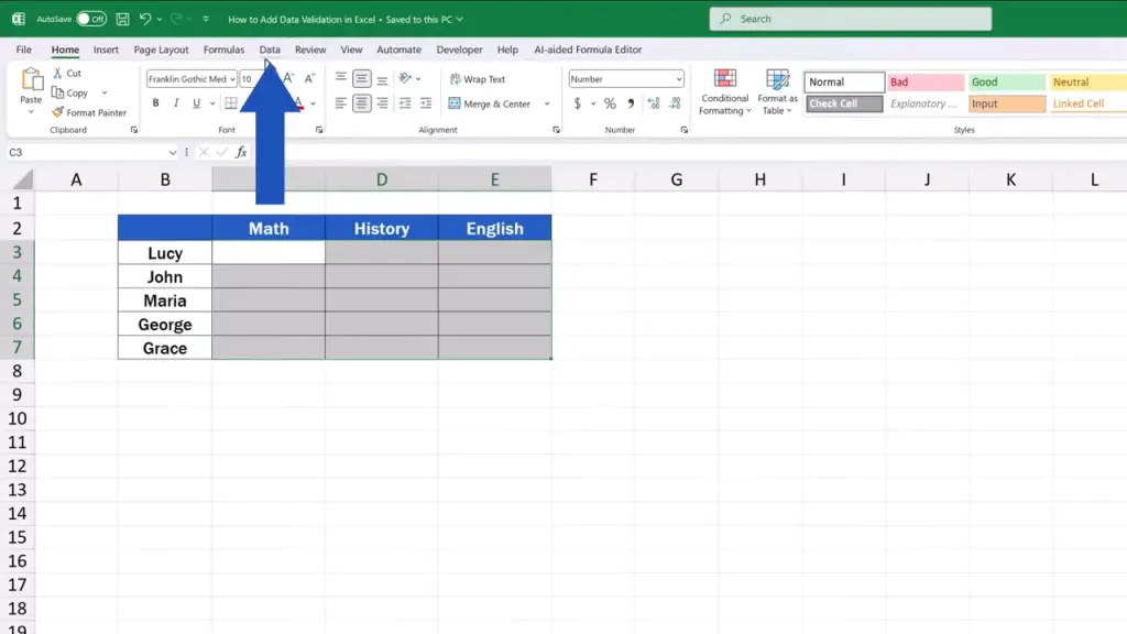
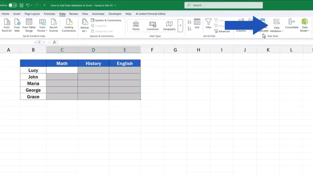
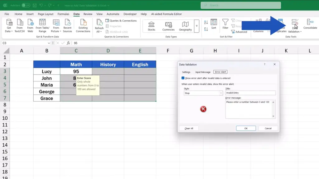
Then we go to the ‘Data’ tab where we find the section ‘Data Tools’. We click on the button ‘Data Validation’.

A window appears where we can enter our settings.

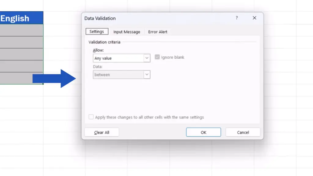
On the tab ‘Settings’, we open the ‘Allow:’ drop-down list. Here we can find all options regarding the value types we can work with, for example, number, date, time, text, and others.

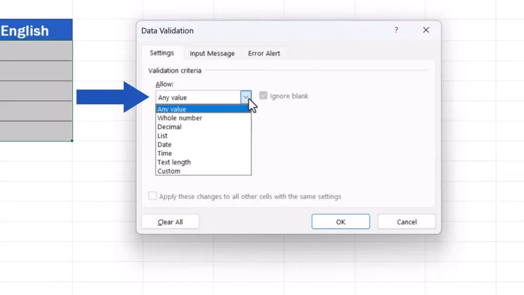
Since we’re going to work with numbers, we select ‘Whole number’ and move on.

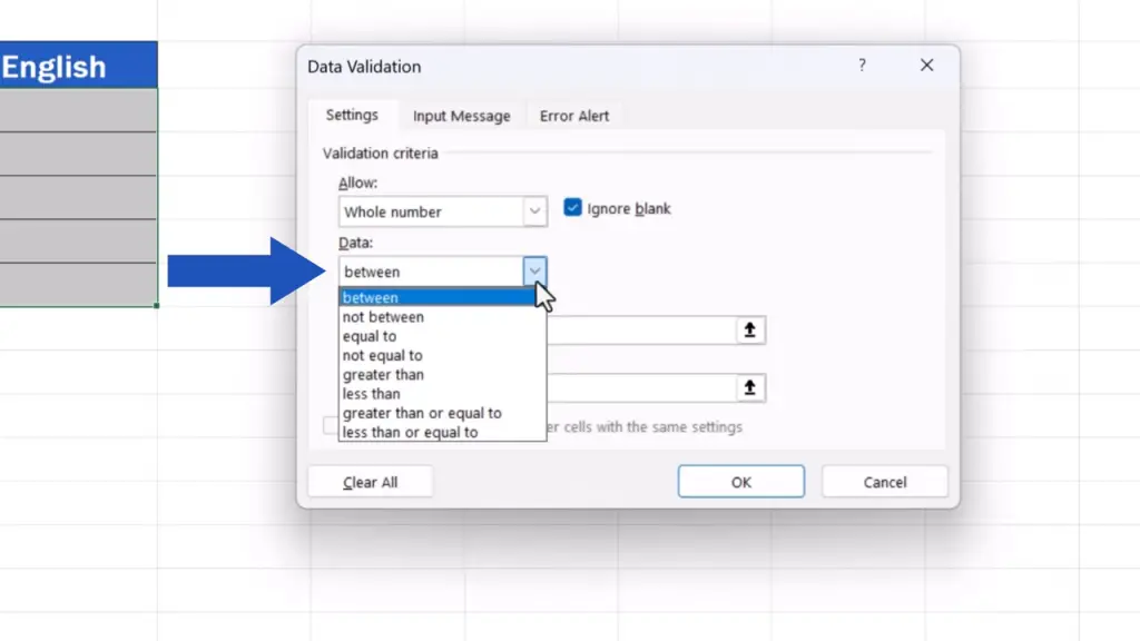
Then there’s a ‘Data:’ entry with a drop-down list, too. This includes various conditions applicable to the relevant value types. We choose ‘between’ here, because we want to enter only numbers between 0 and 100.

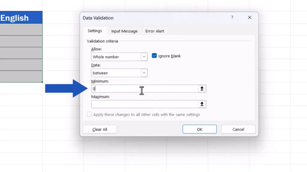
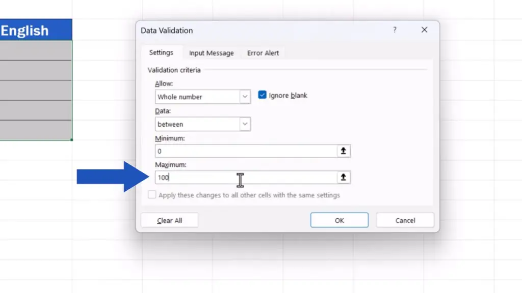
Once we’ve moved on, we can specify the minimum and maximum value, minimum being 0 and maximum 100 in our case.

How to Set Up an Input Message in Excel

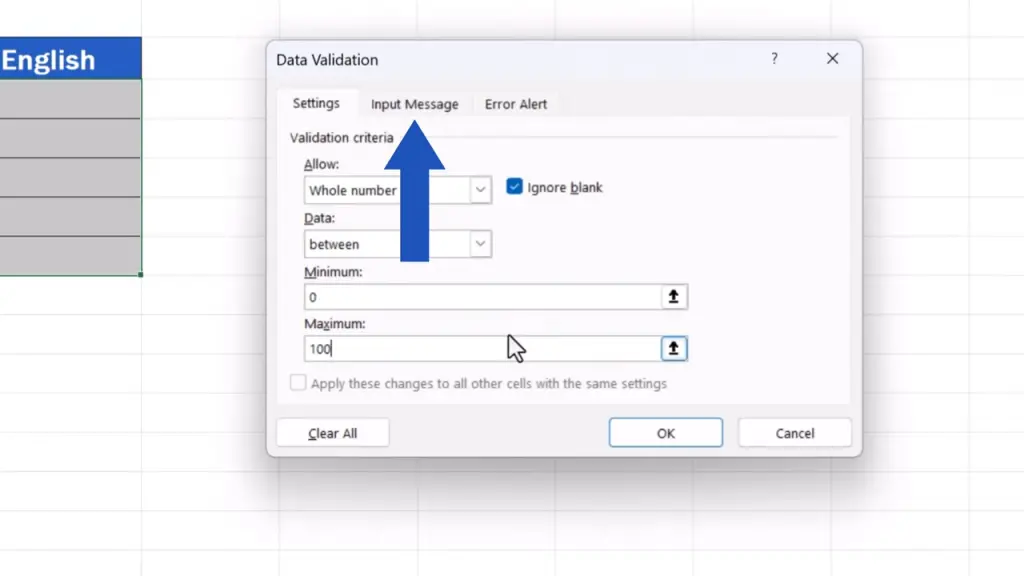
Now, we change tabs and move to ‘Input Message’.

Here we can set a specific prompt that appears every time someone clicks on the cell. If you don’t want this notification to appear, simply untick this box and you don’t have to fill it in at all.

However, we’re going to use this prompt now, so that we could have a look at how everything around Data Validation works.

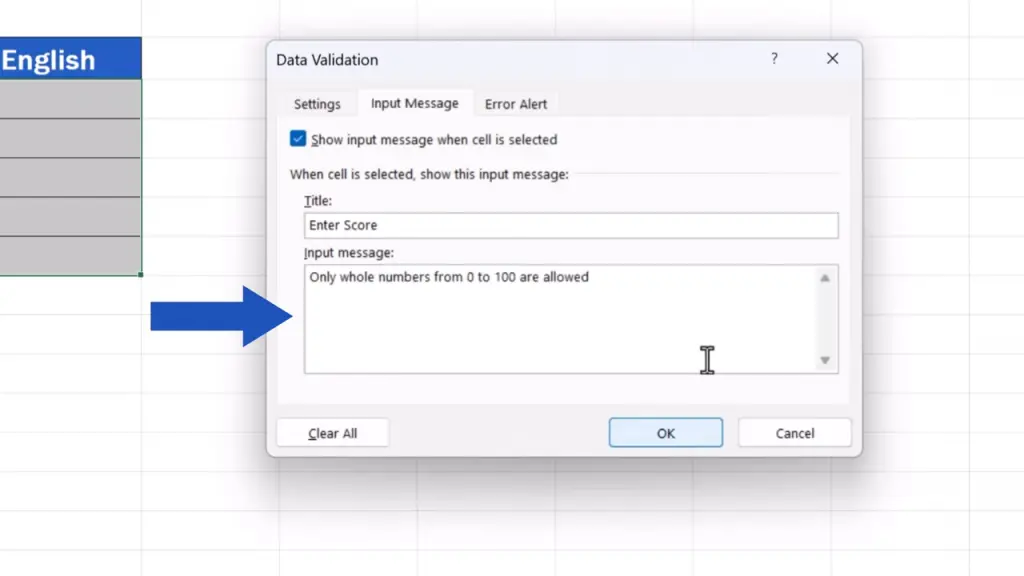
For ‘Title:’, type in ‘Enter Score’.

And for ‘Input message:’, we can type in, for example, ‘Only whole numbers from 0 to 100 are allowed’.

This message serves as a prompt for anyone filling the data table. Based on these specifications, they’ll immediately know what data they’re expected to fill in the table.

How to Set Up an Error Message for Invalid Data

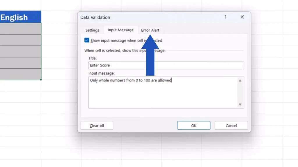
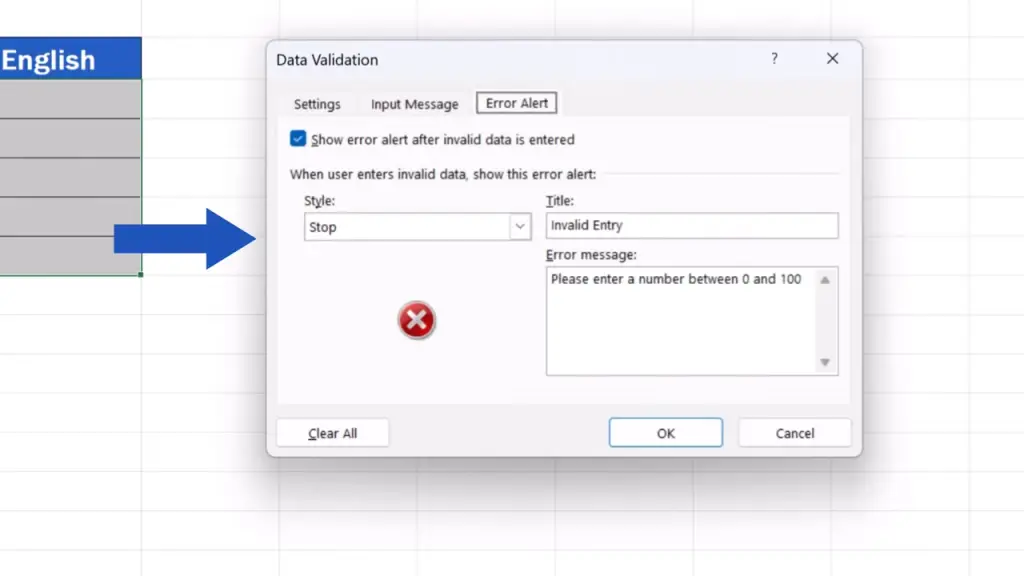
Let’s move on now to the tab ‘Error Alert’.

In this tab we can define an error message which will show if someone enters an incorrect value. Again, it can be turned off by unticking this box up here.

We’ll leave ‘Style:’ on ‘Stop’, which means Excel will block an incorrect data entry. Of course, there are other options in the drop-down list. If needed, you can use them, too.

The title will be ‘Invalid Entry’ and the specific error message will be ‘Please, enter a number between 0 and 100’.

Now, let’s just click on OK and that’s it!

We’re all set now and we can have a look at how Data Validation works in practice.

If we click on any of the selected cells, we’ll see this prompt we just typed in a short while ago. So, we see that we should enter a score within the allowed value range, which is between 0 and 100.

Let’s fill in the score for Mathematics.

We click on the first cell, enter 95, press Enter, and everything goes smoothly.

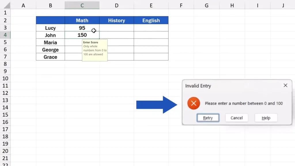
But what if we want to enter 150 into the cell below? Excel blocks us immediately and shows the set error message. So, we see right away that the value we wanted to enter was not correct, as we’ve got to enter a number between 0 and 100.

This is the core of the function Data Validation – to make sure the values entered into a data table by various users match the desirable value types and ranges.

How to Remove Data Validation

And if we don’t need to use Data Validation anymore, we can simply turn the feature off.

Again, we select the relevant cells. Then, we click up here on the ‘Data’ tab, find ‘Data Validation’ one more time, and we’ll see the window with Data Validation settings, again.

Here we click on ‘Clear All’, and press OK, and the settings are all gone, now.

The selected cells are open for any data entry, again.

And before we wrap it up, there’s one important thing to keep in mind.

The Data Validation settings we’ve just seen are great if you want to allow bigger number ranges to be entered into a data table, like we just did, a range from 0 to 100.

If you need the cells to contain just a couple of options, for example, ‘Yes’ or ‘No’, it’s better to use a drop-down list.

And to learn how to do that, watch our separate video tutorial titled ‘How to create a drop-down list in Excel’. The link to the video is in the description below.

Don’t miss out a great opportunity to learn:

If you found this tutorial helpful, give us a like and watch other tutorials by EasyClick Academy. Learn how to use Excel in a quick and easy way!

Is this your first time on EasyClick? We’ll be more than happy to welcome you in our online community. Hit that Subscribe button and join the EasyClickers!

Thanks for watching and I’ll see you in the next tutorial!