How to Calculate the Weighted Average in Excel (using the function SUMPRODUCT)

This tutorial offers a quick and easy way how to calculate a weighted average in Excel.

Are you curious to learn more?

Would you rather watch this tutorial? Click the play button below!

What is the Difference between Weighted and Regular Average

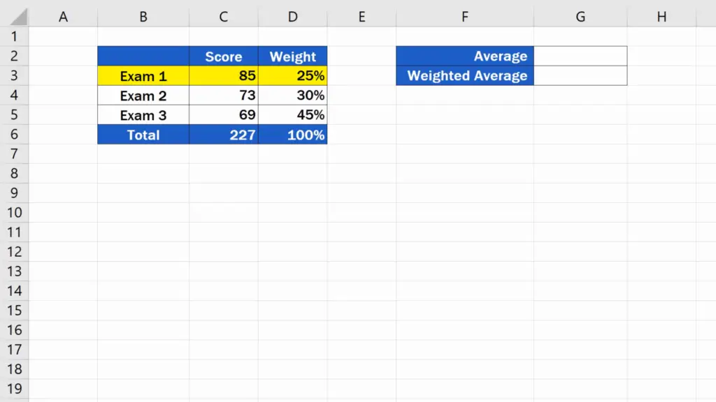
Weighted average is a calculation standardly used if the values for calculating an average have a varying degree of importance. For weighted average, the degree of importance for each value is taken into account. Just like in our example, where the score for each exam has a different weight.

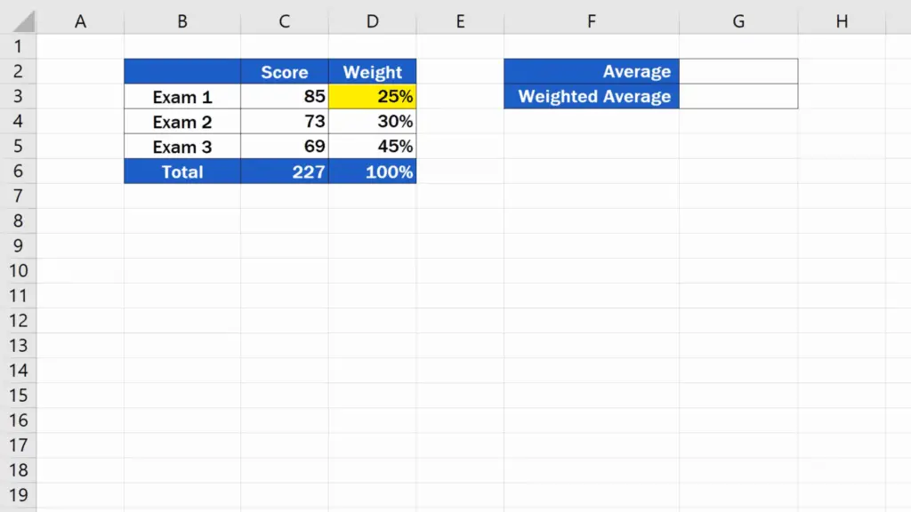
So, here we’ve got the score values and for each value, we’ve got the information on how important it is, which is expressed in per cent.

How to Calculate the Average in a Standard Way

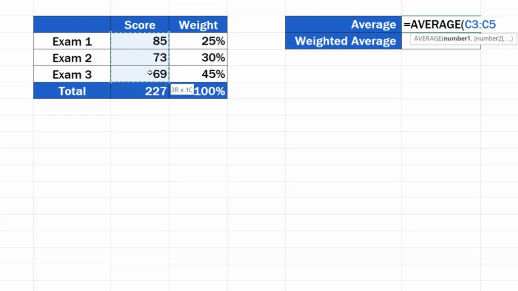
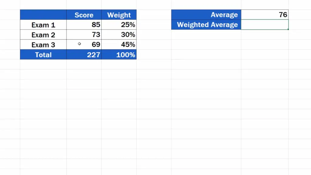
When calculating the regular average, each value we use for calculation is equally important, they have the same weight. To calculate the average in a standard way, we can use the function ‘Average’. We simply enter the values to be used in this calculation and it’s as easy as that. To learn more about this function, EasyClick Academy prepared a separate tutorial the link to which you can find in the list below.

But in today’s tutorial, we’ll focus on how to calculate the weighted average. For this calculation, as you might already suspect, we’ll need to use a different function, specifically SUMPRODUCT.

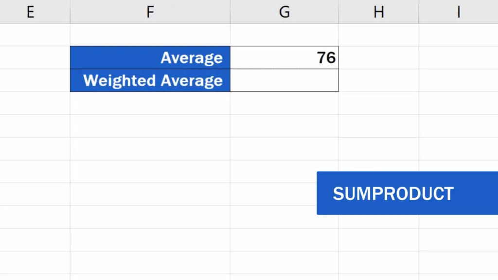
Let’s have a closer look at this function and see how we can calculate the weighted average of these values using SUMPRODUCT.

How to Calculate the Weighted Average Using the SUMPRODUCT Function

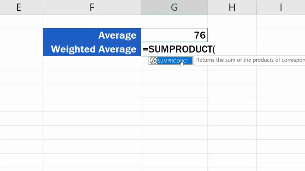
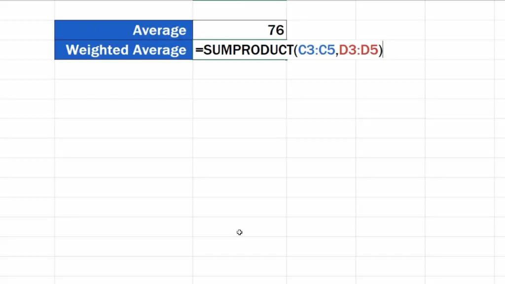
First, click into the cell where you want to calculate the weighted average. Enter the equal sign and start typing ‘SUMPRODUCT’.

Excel will look it up, so we can simply click on it and fill in the data.

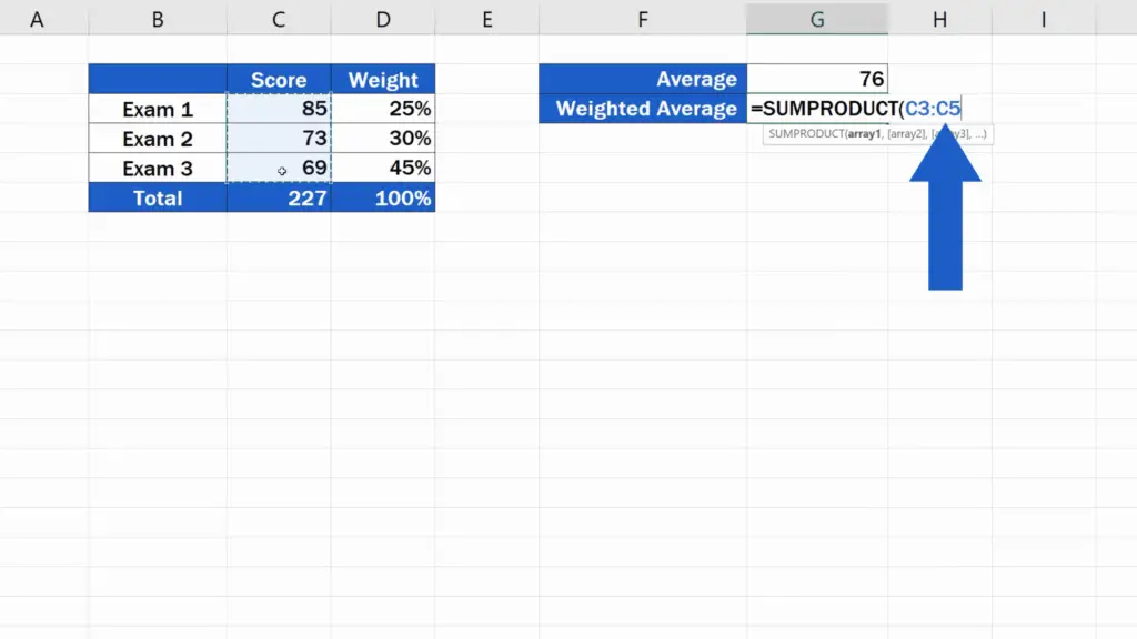
First come the score values, the exam results from column C. We select all values we want to include in the calculation, so we highlight the whole area with these figures. As you can see, Excel entered the coordinates of the selected area into the formula.

Now we add a comma, and the data on weight of particular values should follow. Again, we select the whole area marking the weight of the values, and again, Excel included the reference to the whole range in the formula.

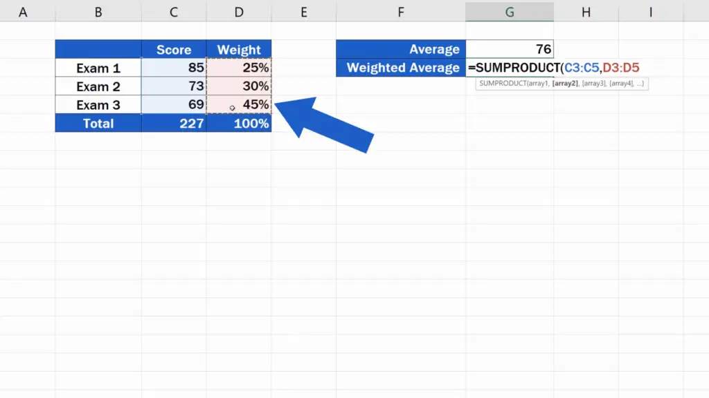
As soon as we’ve got the Score and the Weight data defined, we close the brackets and move on to the next part.

Here, we need to divide the whole calculation with the sum of all Weight values we’re working with. So, we’ll enter the division slash, type in ‘SUM’ and fill the data from the section ‘Weight’ in the brackets again.

We close the brackets, hit ‘Enter’ and that’s all it takes!

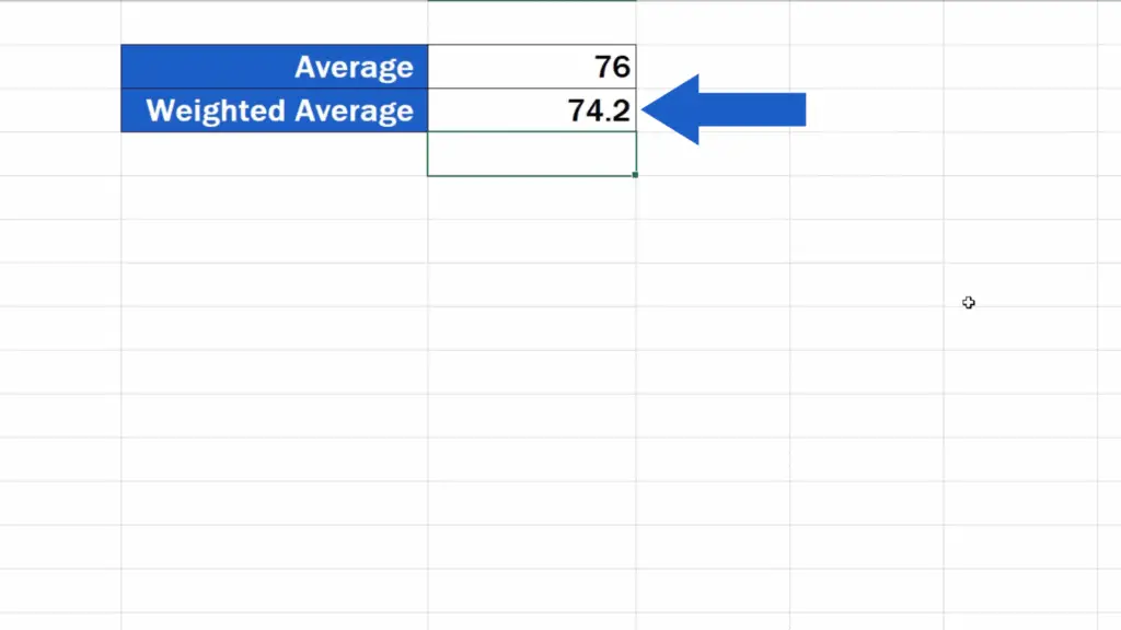
Here’s the weighted average calculated in a quick, easy and effective way, which works with any amount of data you need to process.

Don’t miss out a great opportunity to learn:

• How to Calculate an Average in Excel
• How to Calculate Percentage Increase in Excel (The Right Way)
• How to Change Negative Numbers to Positive in Excel

If you found this tutorial helpful, give us a like and watch other tutorials by EasyClick Academy. Learn how to use Excel in a quick and easy way!

Is this your first time on EasyClick? We’ll be more than happy to welcome you in our online community. Hit that Subscribe button and join the EasyClickers!

Thanks for watching and I’ll see you in the next tutorial!