How to Change Chart Style in Excel

This tutorial covers how to change chart style in Excel. In a very simple way, you can change the style of your charts as you need.

Let’s get into it!

Would you rather watch this tutorial? Click the play button below!

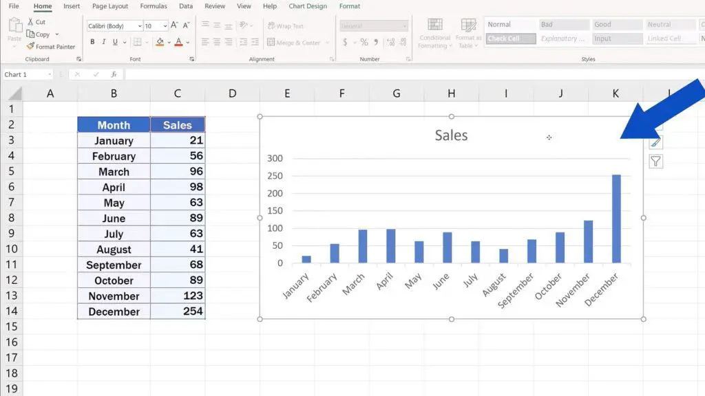
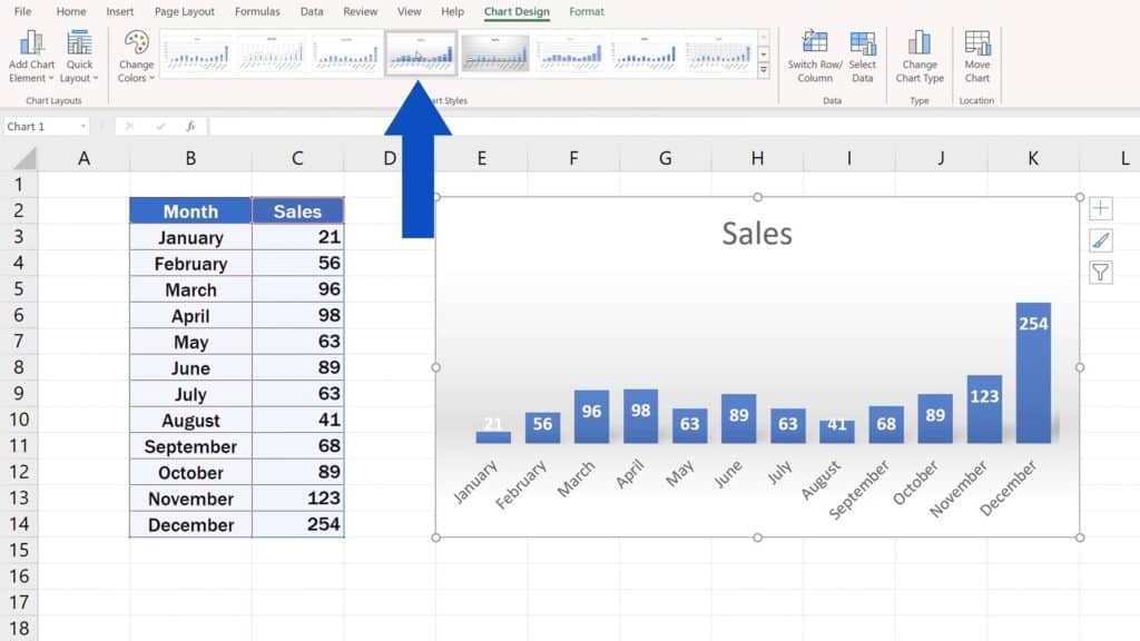
If you need to change chart style, select the chart area first by clicking on it.

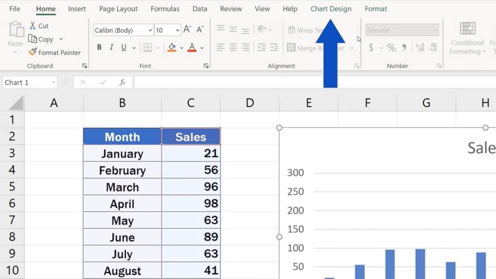
On the top horizontal bar called ‘Ribbon’, you will see the tab ‘Chart Design’.

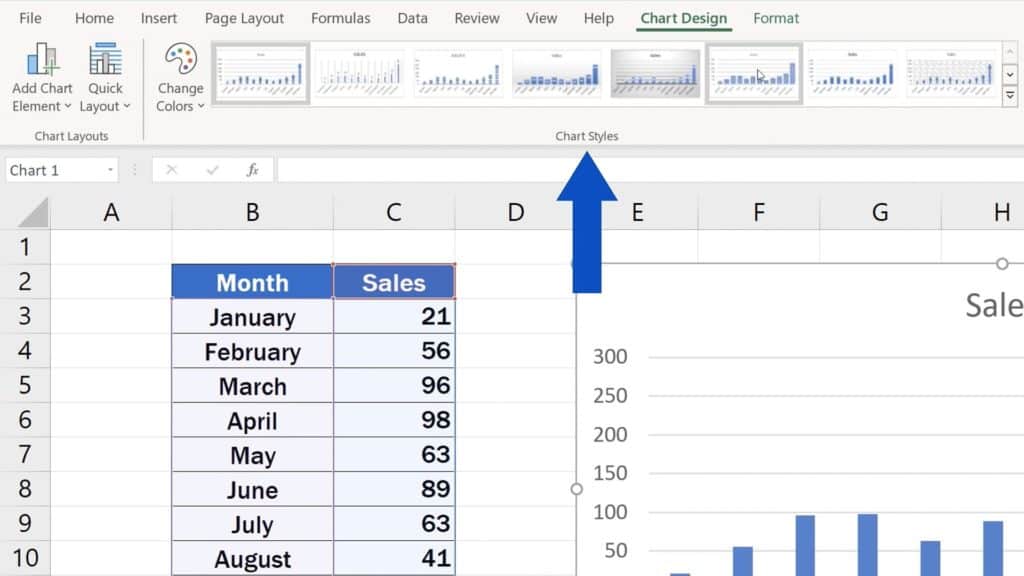
Go to the tab and in the section ‘Chart Styles’, you can pick any style you like from the offered menu of styles and effects.

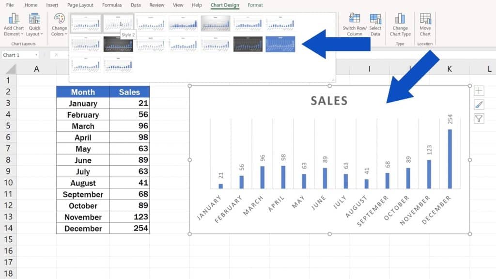
Let’s choose this one for now and let’s move on.

How to Change the Chart Color in Excel

Once you find the style you like, but you don’t like the colour, you can click on the option ‘Change Colors’ here.

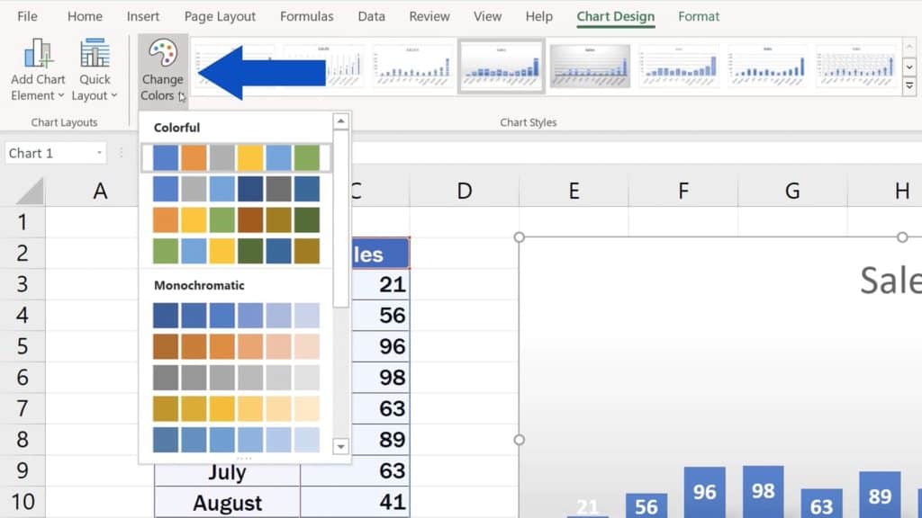
In this part, you’ll get to choose from various colour possibilities Excel offers. We’ll go for this green.

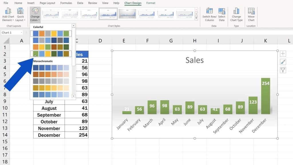
If you can’t find the colour you’re looking for in the option ‘Change Colors’, there’s still a way how you can change the chart colour to the one you need. See our tutorial on how to change chart colour in Excel, which will tell you exactly how you can do it. The link is in the list below.

Don’t miss out a great opportunity to learn:

• How to Add a Title to a Chart in Excel (In 3 Easy Clicks)
• How to Add Axis Titles in Excel
• How to Add a Trendline in Excel

If you found this tutorial helpful, give us a like and watch other video tutorials by EasyClick Academy. Learn how to use Excel in a quick and easy way!

Is this your first time on EasyClick? We’ll be more than happy to welcome you in our online community. Hit that Subscribe button and join the EasyClickers!

Thanks for watching and I’ll see you in the next tutorial!