How to Convert Currency in Excel

Today we’re going to talk about the easiest way how to convert currency in Excel. First, we’re going to have a look at how we can conveniently obtain the information on the current exchange rates for various currencies. Then, we’re going to make a simple currency exchange calculator to convert any amount from one currency to another.

Ready to start?

Contents hide

1 How To Refresh Exchange Rates Automatically or Manually

2 How To Calculate Currency Conversion Correctly

3 How To Refresh Exchange Rates Automatically or Manually

How To Refresh Exchange Rates Automatically or Manually

To convert an amount from one currency to another in Excel, first, we need to define a so-called currency pair which we’ll be working with.

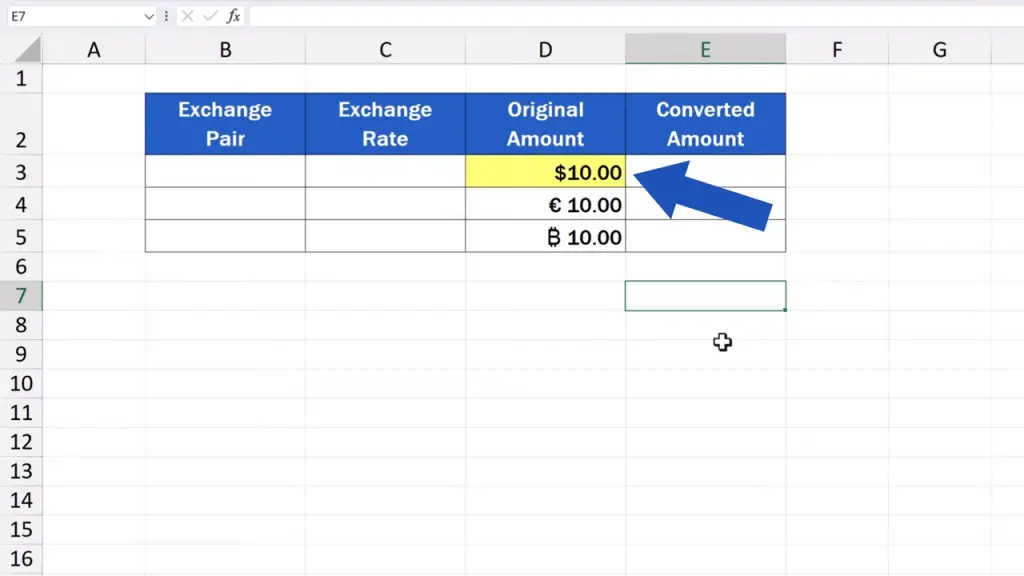
The original amount in D3 is in the U.S. dollars and let’s say that we want this amount converted to euros.

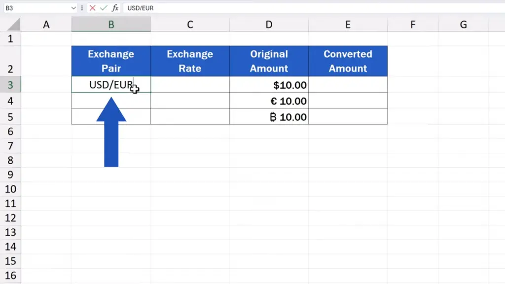
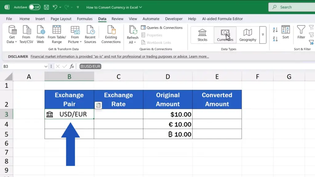
So, the first currency pair to be entered to B3 is going to look like this: USD/EUR. Everything needs to be typed in capitals, with no spaces, divided by a forward slash.

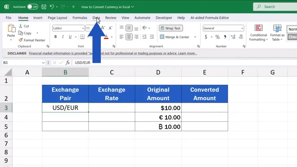
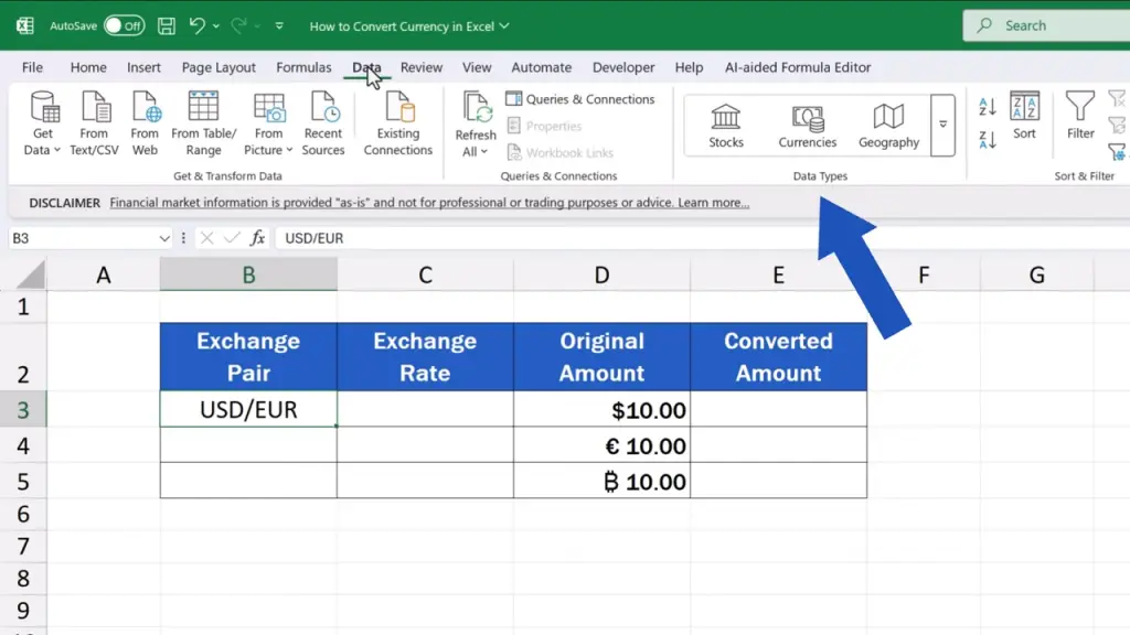
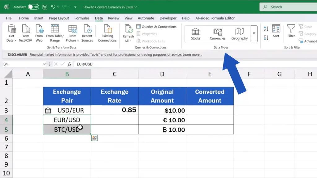
As soon as we’ve got the pair specified like this, we click on the cell, then we go to the ‘Data’ tab, and in the section ‘Data Types’, we select ‘Currency’.

Excel immediately recognises the currency pair and changes this simple cell to a cell with the designated data type. That means that the cell is now connected to an online database from which Excel can retrieve the most up-to-date data.

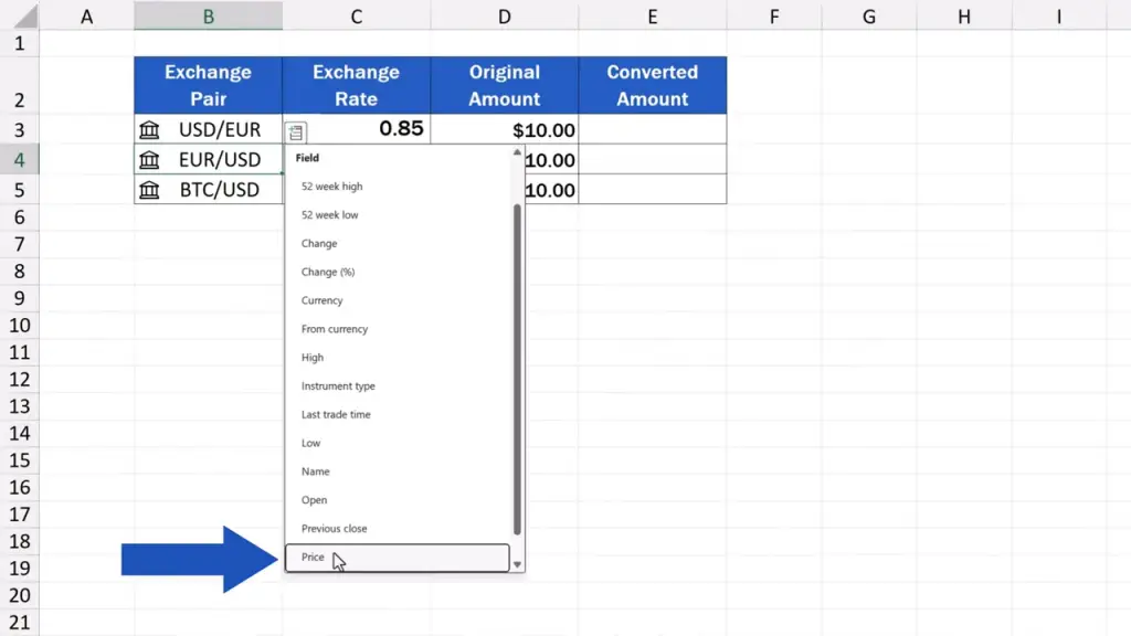
You can find the data when you click on this little icon next to the cell.

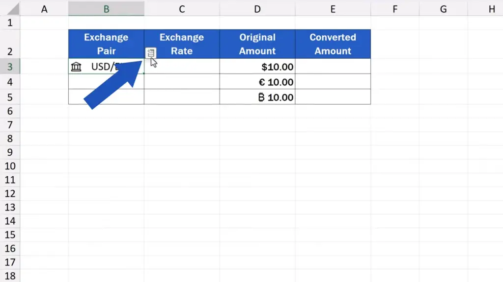
When we click on it, we can choose what kind of information relevant to the currency pair we want Excel to retrieve. We’re interested in ‘Price’.

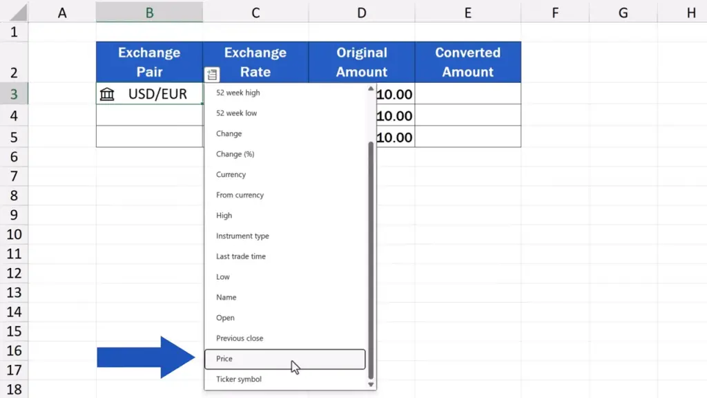
And Excel has immediately entered the current exchange rate for this currency pair in the column on the right. When we were making this video, the current exchange rate for the pair was 0.85, which means that for a dollar we get 85 euro cents.

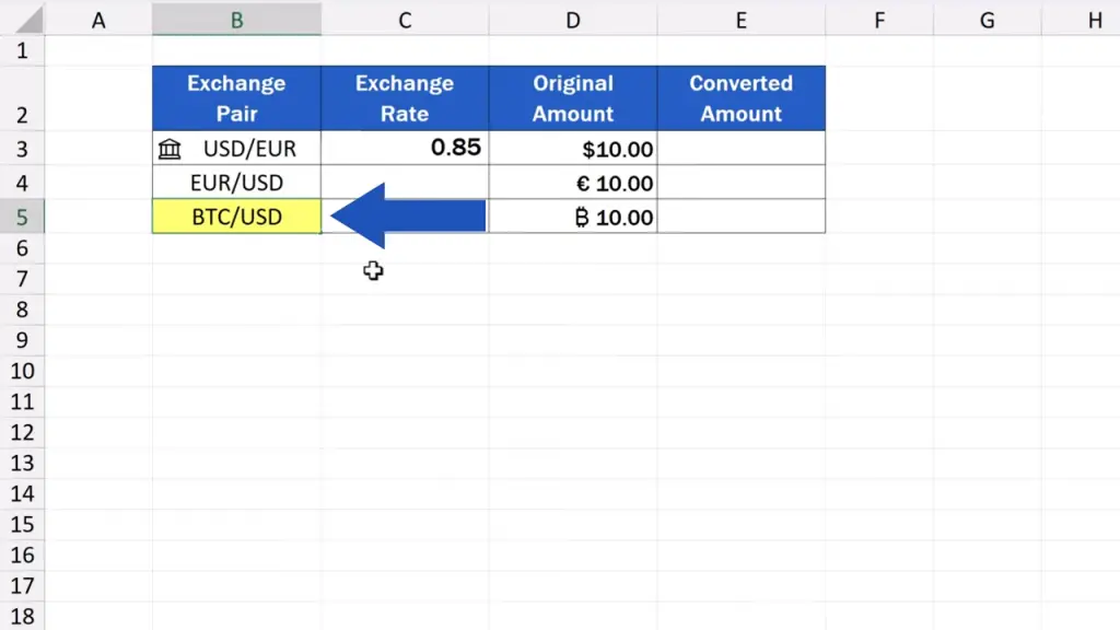
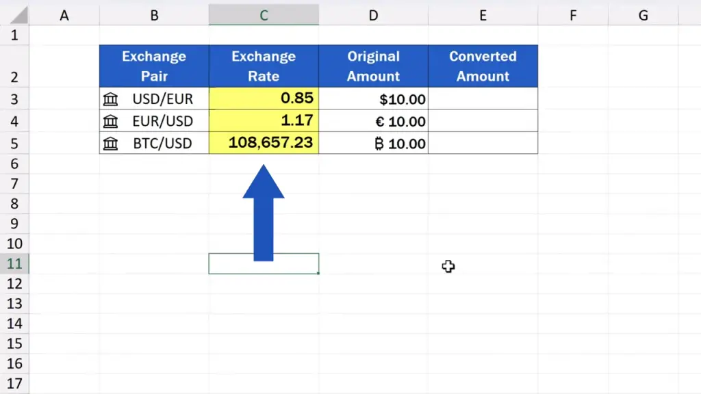
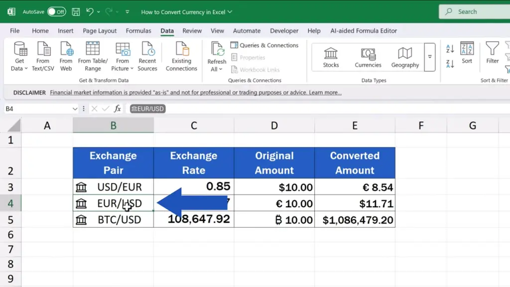
The same way we can identify more currency pairs, in our case it’ll be two more. So, in B4 we enter the currency pair Euro to U.S. Dollar.

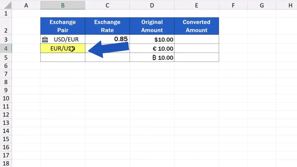
And in B5 we can have the Bitcoin and the U.S. Dollar.

This is how we can enter any currency pair and as many of them as we need.

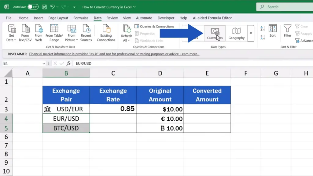
Then, we assign the data type to the cells, just as we did a while ago. We select both, then we go to the ‘Data’ tab, and in the section ‘Data Types’, we select ‘Currency’.

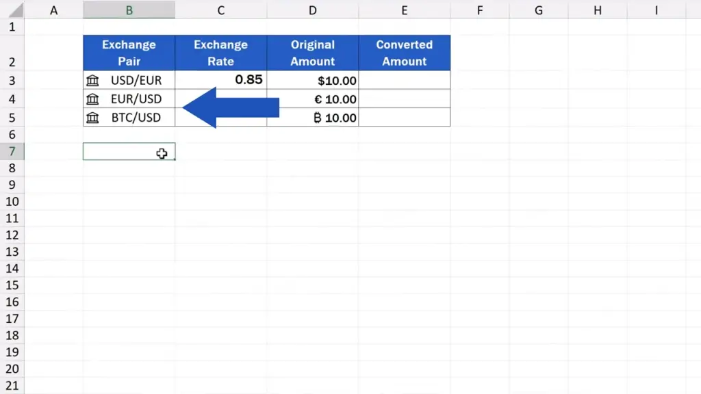
When done, we make the prices show in the column on the right, and that’s it. The exchange rates show for every currency pair.

How To Calculate Currency Conversion Correctly

Let’s move on.

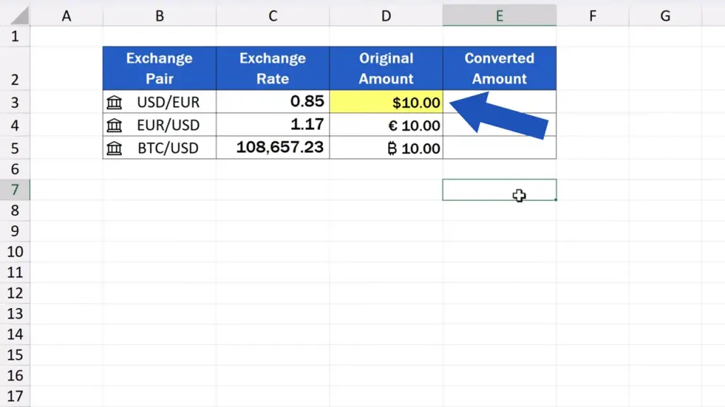
Now, we can have a look at a simple formula that will actually perform the conversion from one currency to the other.

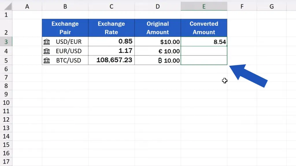
The original amount in D3 is 10 U.S. Dollars.

So, in E3, we type the equal sign and then D3 and an asterisk followed by C3, which will multiply the amount in D3 with the exchange rate in C3. That will calculate how much the original amount is in euros.

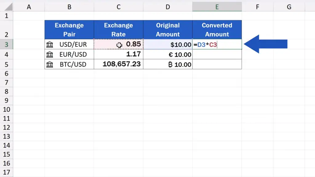
We can copy the same formula to these two cells we’ve got left and that’s it. We’re finished with the conversion.

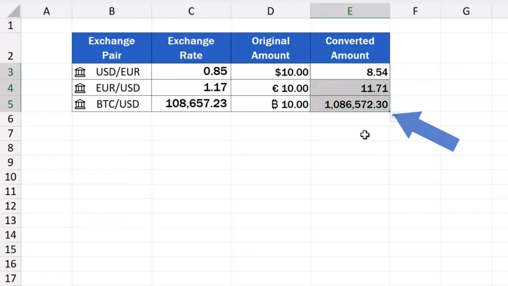
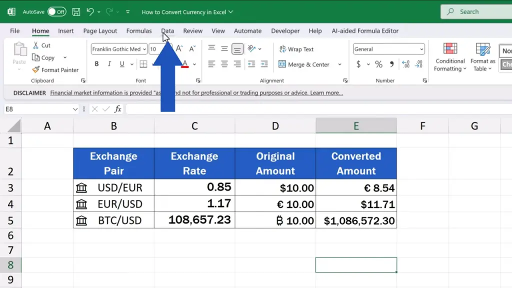
Now, we can format the figures in the column ‘Converted Amount’, so that they would contain the symbols of the currencies.

We can do this through a handy ‘Format Painter’ feature. If you don’t know how to use the ‘Format Painter’ feature, make sure to check out our video tutorial How to Copy Formatting in Excel (The Quickest Way)! The link to the video is in the description below.

And here’s another important bit of information you might be interested in.

The exchange rates we’re working with are not randomly scraped from the Internet. Excel uses a reliable and established source with which Microsoft partners, so you can be sure that these values are always up-to-date and dependable.

How To Refresh Exchange Rates Automatically or Manually

And that’s not all!

Let’s have a look at the last important part you should know and that is how to keep the exchange rates up to date.

There are three ways.

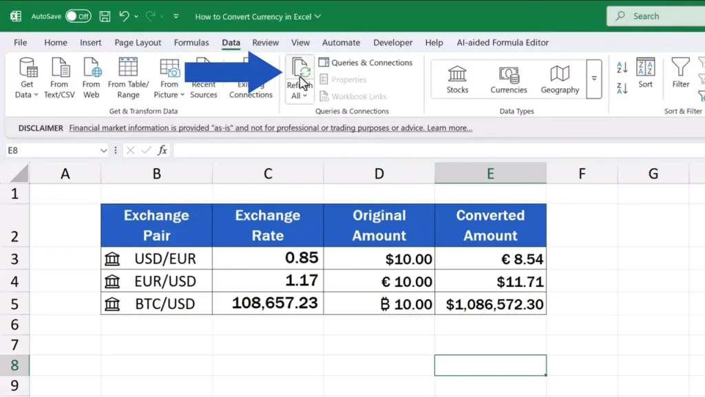
The first one is to refresh the rates manually, which can be done anytime you need. Simply press the button ‘Refresh All’ up here in the ‘Data’ tab and all the rates will be updated.

The latter two are automatic and you can set them the following way.

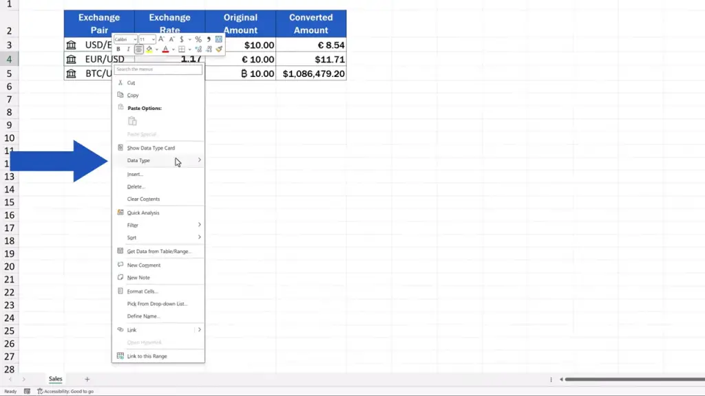
First, right-click on the cell containing the currency pair, for example Euro to U.S. Dollar.

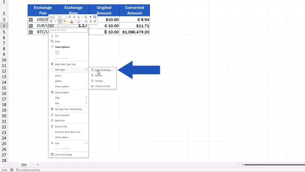
Then select the option ‘Data Type’ to open ‘Refresh Settings’.

On the right, you’ll see a pane with options. Click on ‘Stocks’ and we can see automatic options to refresh the rates.

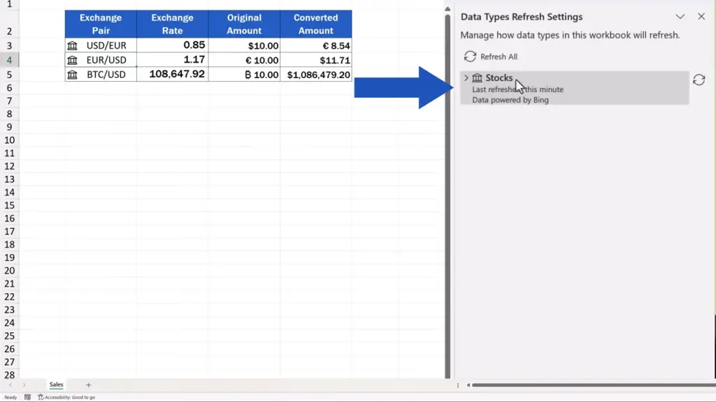
The data can get refreshed every five minutes or just when the file is opened.

Or we can simply keep the manual setting to refresh the rates, which we’ve just seen.

Select the option that suits you best and that’s it!

This way, you can conveniently use the most up-to-date exchange rates in any data tables.

And if you’d like to know how to be always up to date with the current stock prices, make sure to watch our video tutorial on How to Get Stock Prices in Excel. We’ve included the link to the video in the description below, too.

Don’t miss out a great opportunity to learn:

If you found this tutorial helpful, give us a like and watch other tutorials by EasyClick Academy. Learn how to use Excel in a quick and easy way!

Is this your first time on EasyClick? We’ll be more than happy to welcome you in our online community. Hit that Subscribe button and join the EasyClickers!

Thanks for watching and I’ll see you in the next tutorial!