How to Freeze Multiple Rows in Excel (Quick and Easy)

Today we’ll have a look at how to freeze multiple rows in Excel, specifically, how to freeze and unfreeze the first two rows. You’ll be able to use the same way to freeze any number of rows, according to what you need.

Let’s get into it!

How to Define which Section of a Data Table We Want to Freeze

To freeze multiple rows, first we need to define which section of a data table we want to freeze.

And that’s done through the cell cursor.

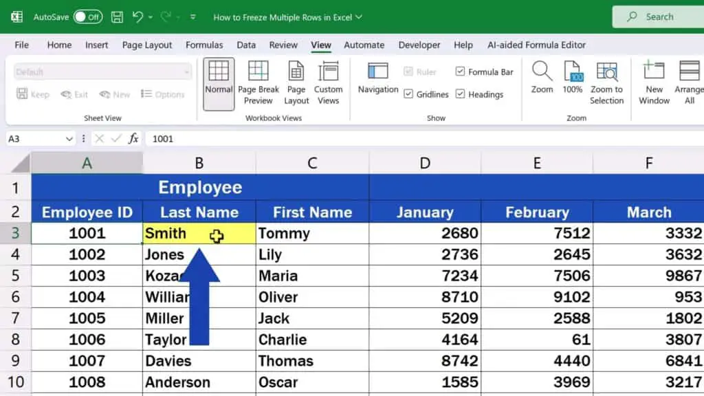
Let’s say we want to freeze just these two rows, here at the top. No columns.

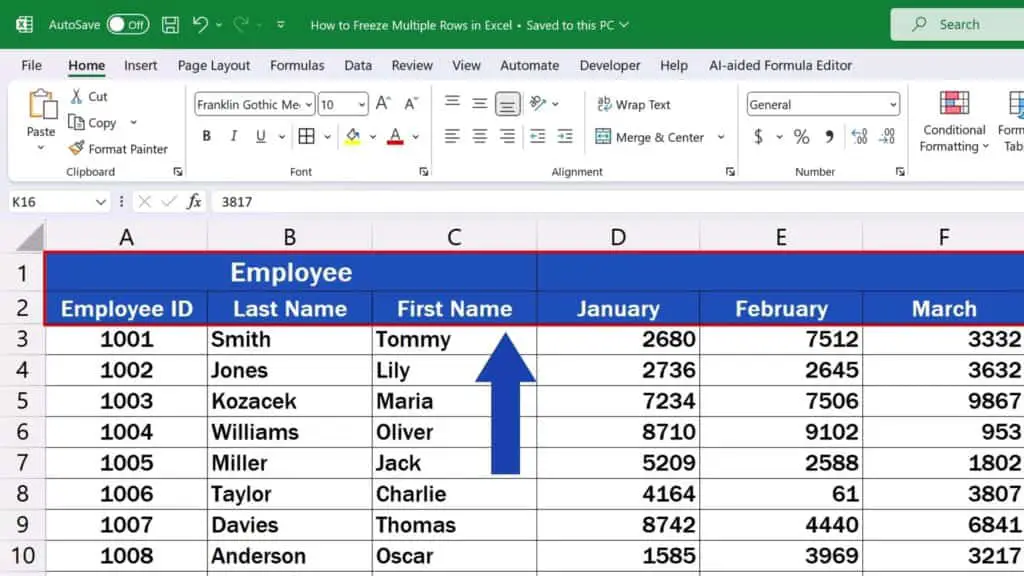
We click on the cell A3, which means all the rows above the cell and all the columns to the left of the cell will be frozen.

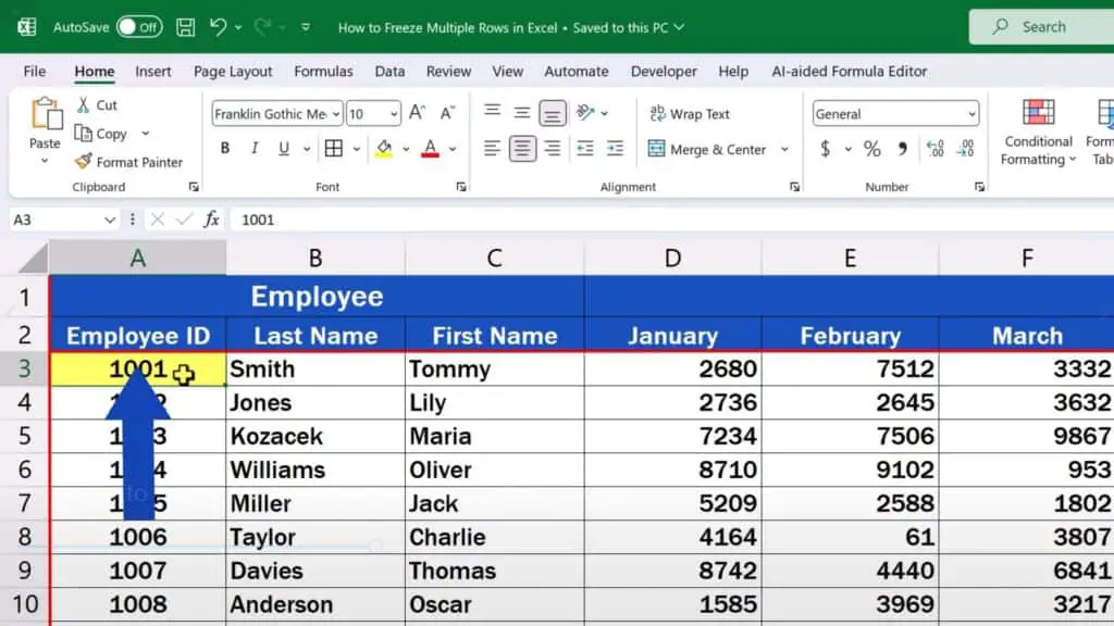
Here it’ll be the first two rows and no columns, because there are none to the left of column A.

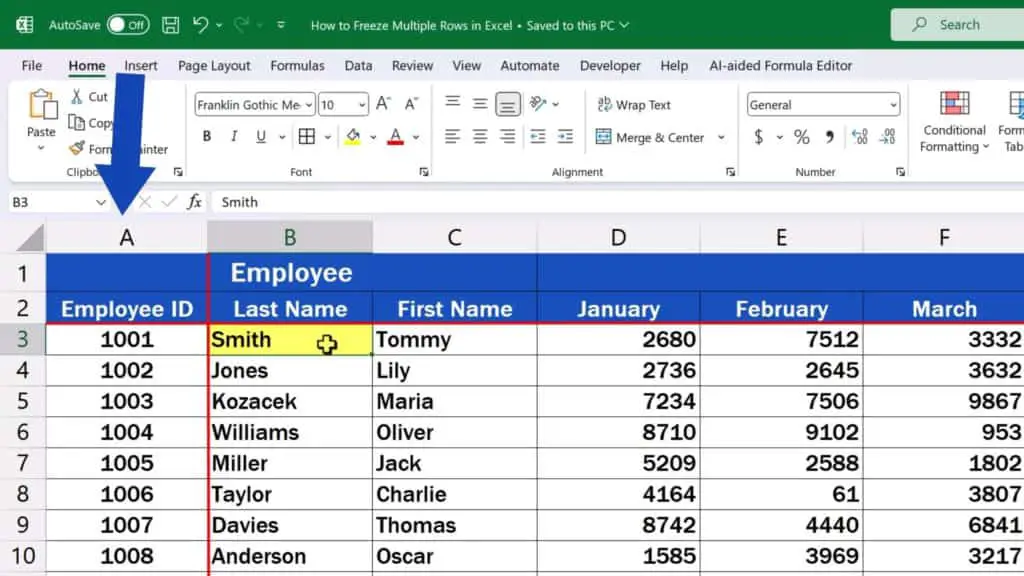
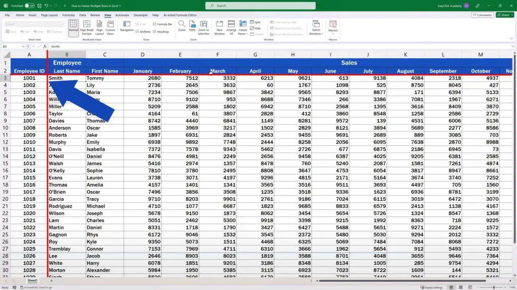
If we set the cell cursor to B3, rows 1 and 2 together with column A will be frozen. So, keep in mind – all the rows above and all the columns to the left of the selected cell.

But now we want to freeze just the first two rows, so we click on A3.

Once this is done, click on the ‘View’ tab, then find ‘Freeze Panes’ and click on it.

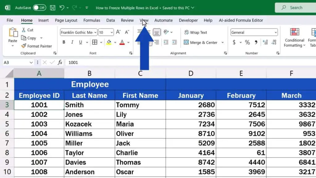
Since we’ve defined the section to freeze, we click on the option ‘Freeze Panes’, which freezes exactly the defined part of the data table – our current selection.

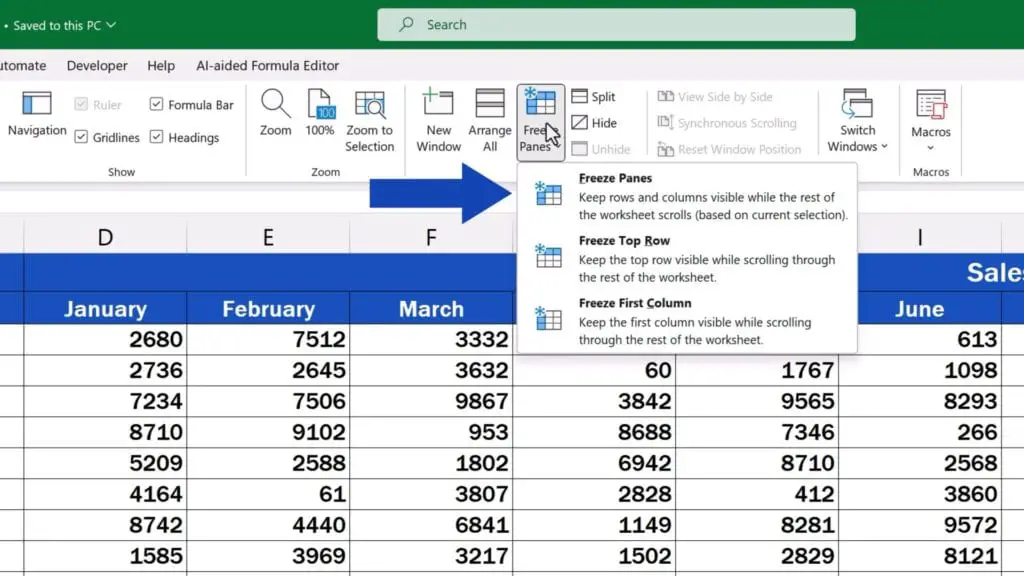
If you need to freeze just the top row or the first column, you can find the options right below this one.

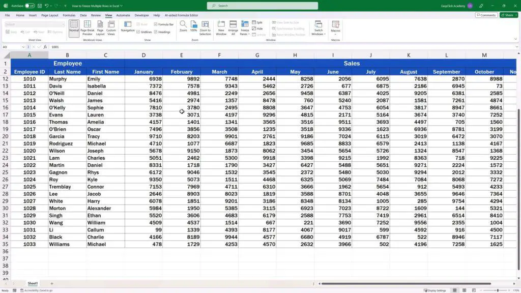
Now we’re going to click on ‘Freeze Panes’ and here are the first two rows of the table frozen – just as we wanted! If we keep scrolling down, these rows stay visible on the screen.

How to Unfreeze Panes

To undo this setting, click on ‘Freeze Panes’ where you can select ‘Unfreeze Panes’.

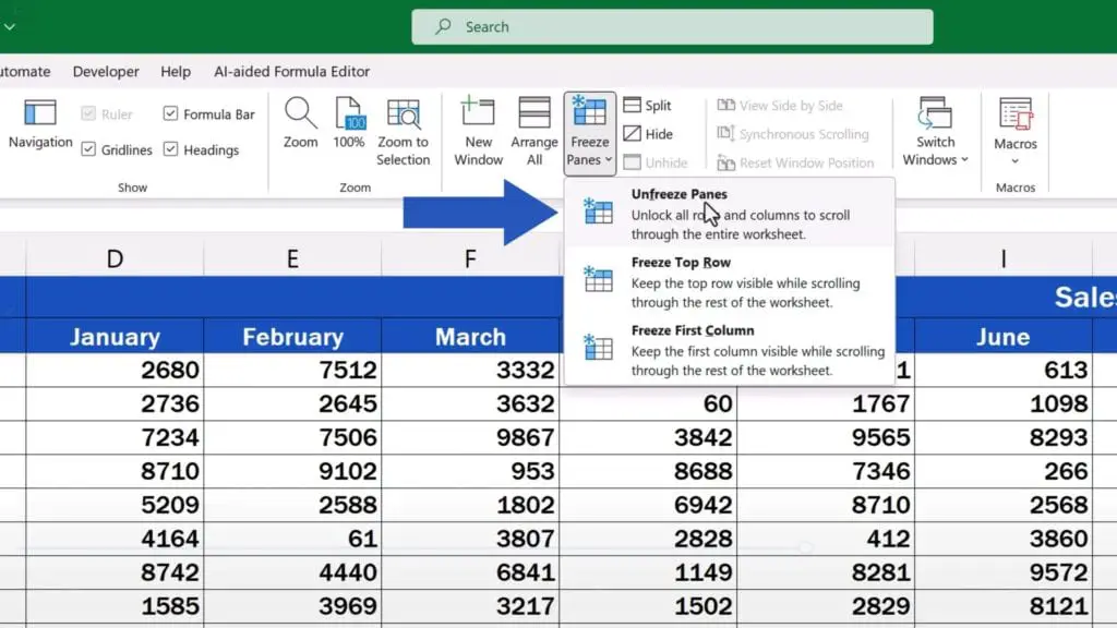
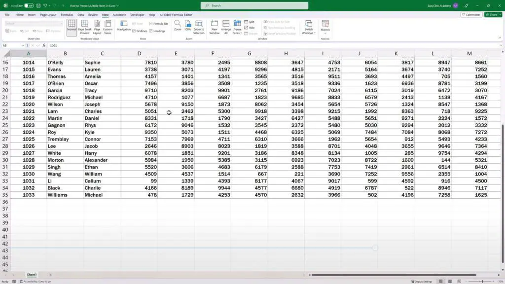
And that’s it! None of the rows is now frozen.

Just to see what would happen if we set the cell cursor on B3, as we mentioned a while ago – once we click to freeze panes, rows 1 and 2 and column A stay visible when scrolling through the table.

This way you can freeze any selection of rows and columns in a data table, depending on what you need!

Don’t miss out a great opportunity to learn:

• How to Freeze Rows in Excel
• How to Freeze Columns in Excel (A Single or Multiple Columns)
• How to Group Rows in Excel (Automated and Manual Way)

If you found this tutorial helpful, give us a like and watch other tutorials by EasyClick Academy. Learn how to use Excel in a quick and easy way!

Is this your first time on EasyClick? We’ll be more than happy to welcome you in our online community. Hit that Subscribe button and join the EasyClickers!

Thanks for watching and I’ll see you in the next tutorial!