How to Indent in Excel

Welcome!

In this video tutorial, we’re going to have a look at the best way how to indent in Excel. Thanks to indentation, the data in a table will look neat and clearly organised.

Contents hide

1 How to Increase Indent in Excel

2 How to Indent Multiple Cells at Once

3 How to Decrease or Remove Indentation

How to Increase Indent in Excel

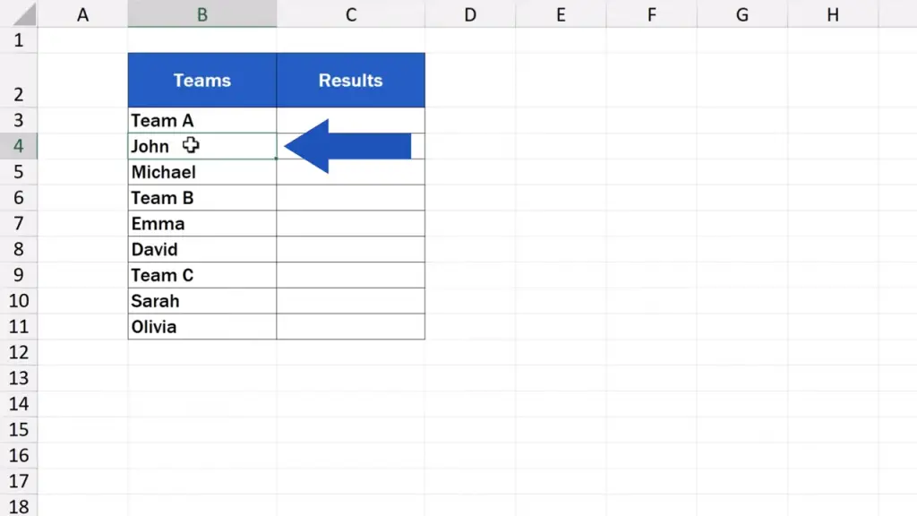
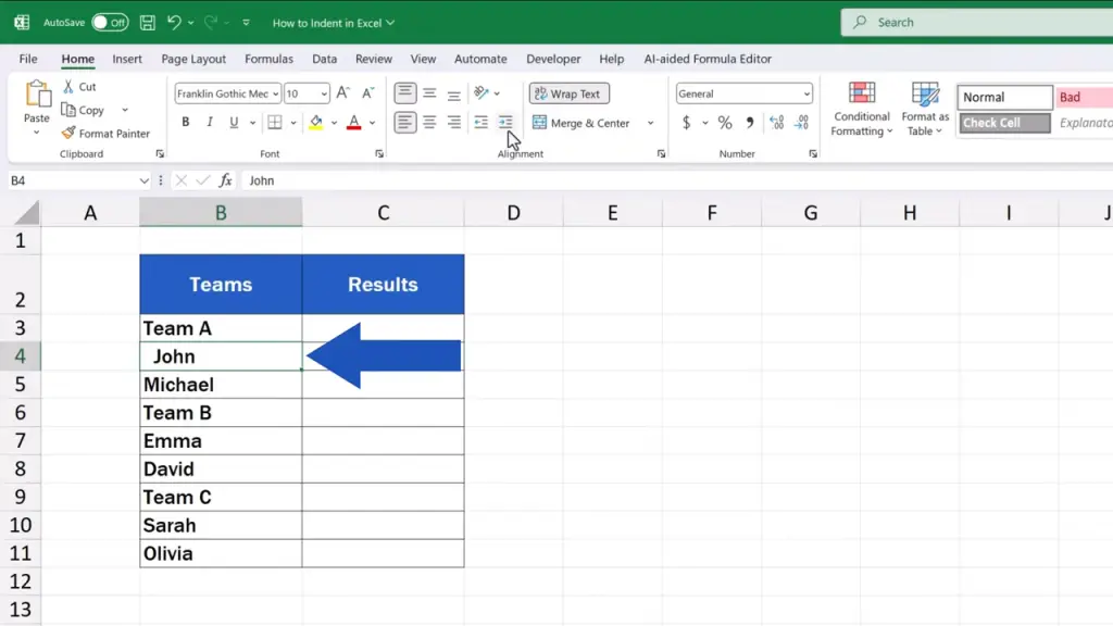
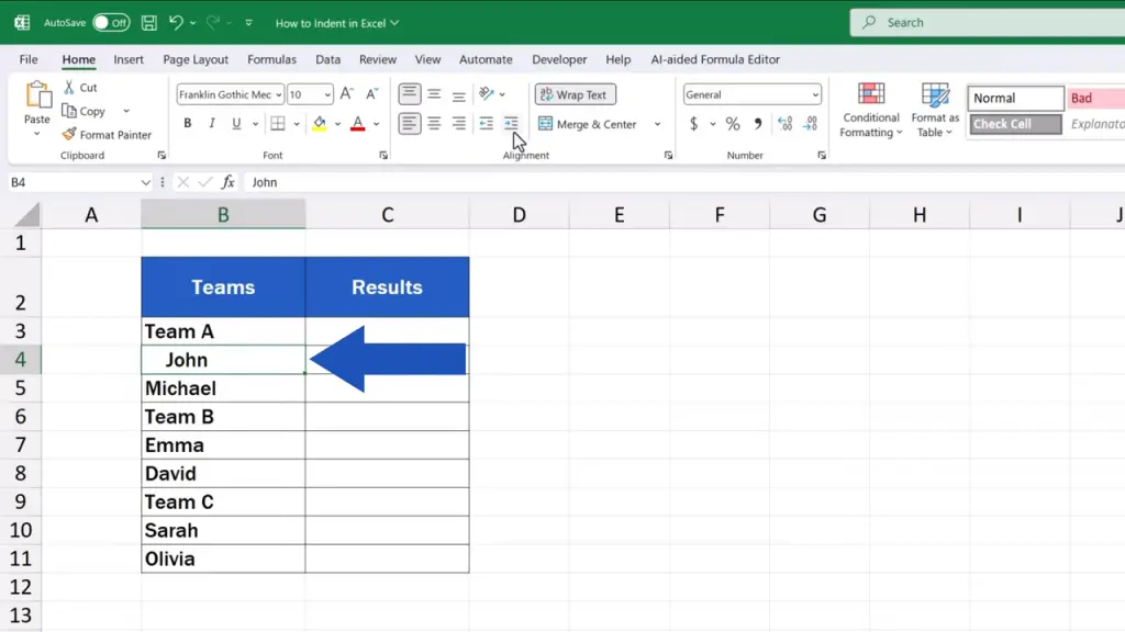
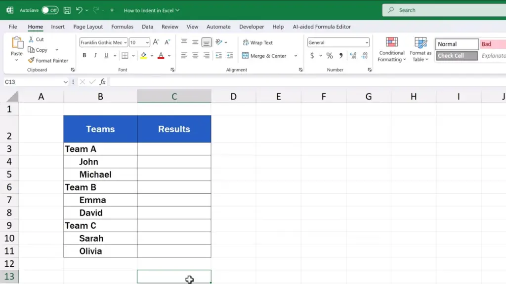
To indent text in Excel, we begin by clicking on the cell we want to alter. Let’s click on the cell B4, which contains the name ‘John’ from Team A.

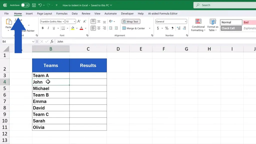
Then, we go to the ‘Home’ tab.

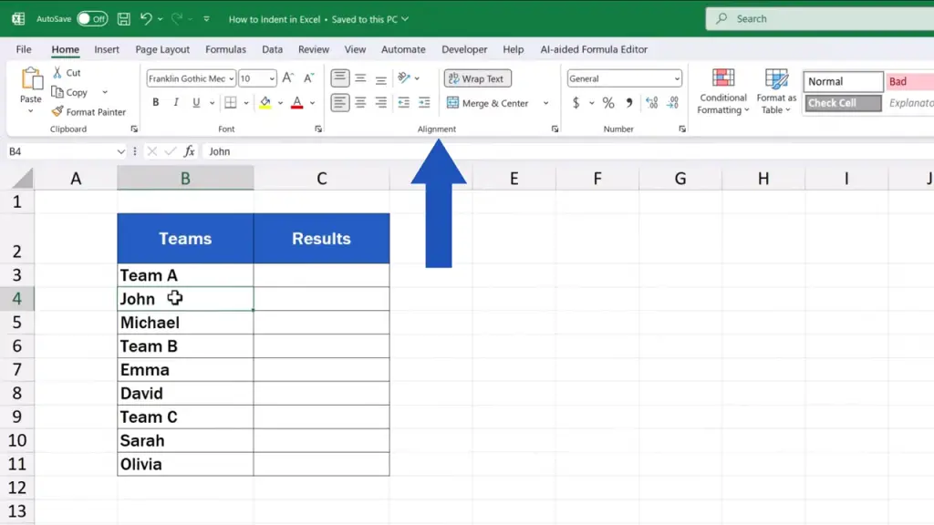
Find the group ‘Alignment’.

And click on ‘Increase Indent’. It’s easily recognisable by the icon showing a right-pointing arrow.

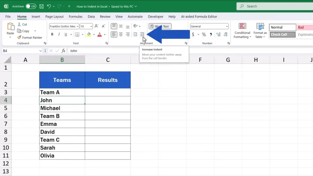
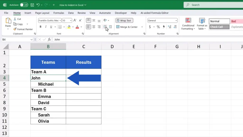
By clicking on the button, the text in the cell moves slightly to the right in an instant.

If we click on ‘Increase Indent’ once again, the text moves further to the right. This way we can set the length of indentation we need.

How to Indent Multiple Cells at Once

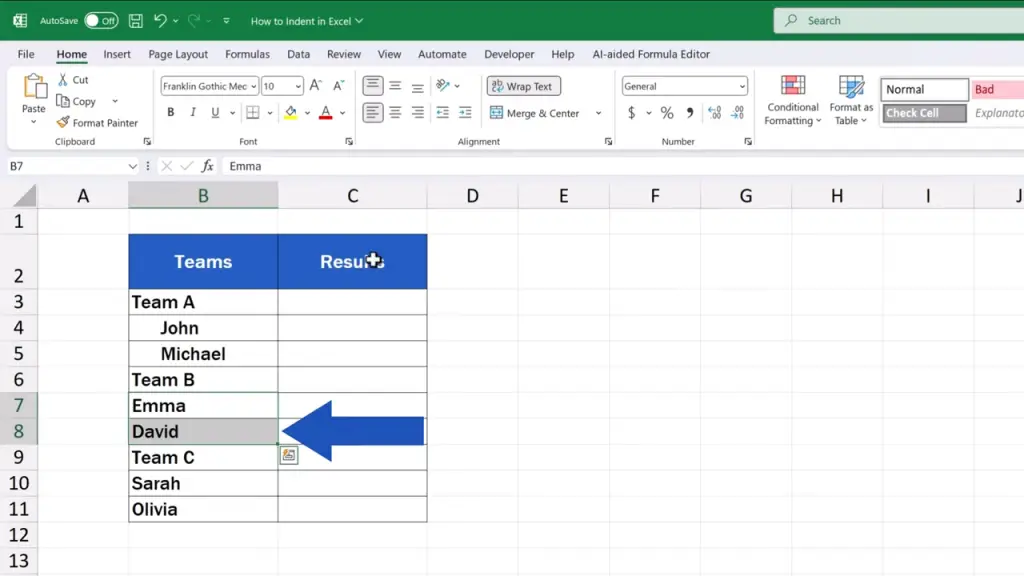
The same way works for cells containing other names. Either we click on each name separately or we can simply select multiple cells at the same time and set the indentation for all of them at once.

How to Decrease or Remove Indentation

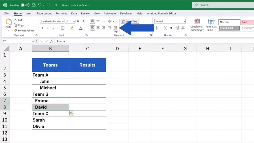
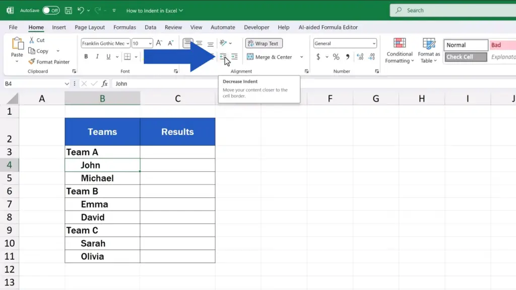
To reduce or remove the indentation, we click on the cell with the indented text, then we click on the ‘Home’ tab and use the button ‘Decrease Indent’ marked with an arrow pointing to the left.

Again, the more we click, the further to the left the text moves until we remove the indentation completely.

To learn more tips and tricks on how to effectively work with text in Excel, watch the whole series of our video tutorials titled ‘How to Work With Text in Excel’. The link to the videos is in the description below.

Don’t miss out a great opportunity to learn:

If you found this tutorial helpful, give us a like and watch other tutorials by EasyClick Academy. Learn how to use Excel in a quick and easy way!

Is this your first time on EasyClick? We’ll be more than happy to welcome you in our online community. Hit that Subscribe button and join the EasyClickers!

Thanks for watching and I’ll see you in the next tutorial!