How to Use Absolute Cell Reference in Excel

This tutorial offers handy advice on how to use absolute cell reference in Excel. We use an absolute cell reference in Excel calculations when we need to keep the reference to a cell in a formula constant.

Let’s have a closer look at what it means in the following example.

Ready to start with some calculations?

Would you rather watch this tutorial? Click the play button below!

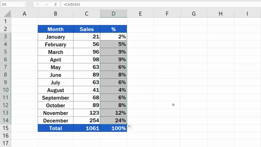
We’ve got a table with the information on sales for each month and down below, there’s the total. Let’s say we need to calculate what portion of the total sales the values for each month represent, in percent.

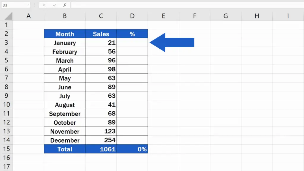
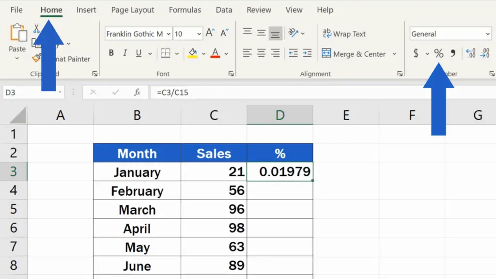
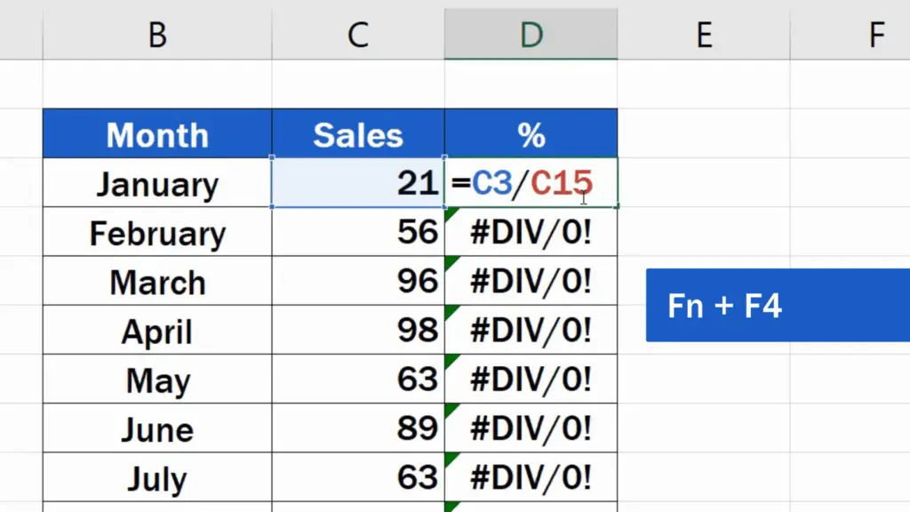
First, find the cell D3, type in the equal sign and divide the sales for that particular month (the information in the cell C3) with the total sales (cell C15).

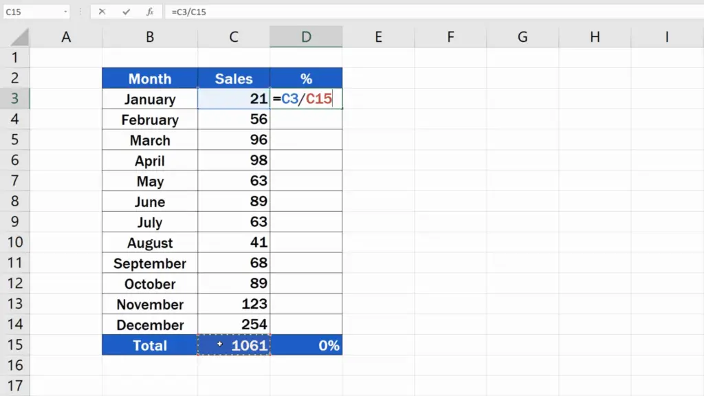
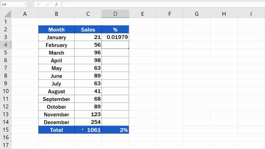
Click on Enter and check the result.

How to Format the Cell Properly

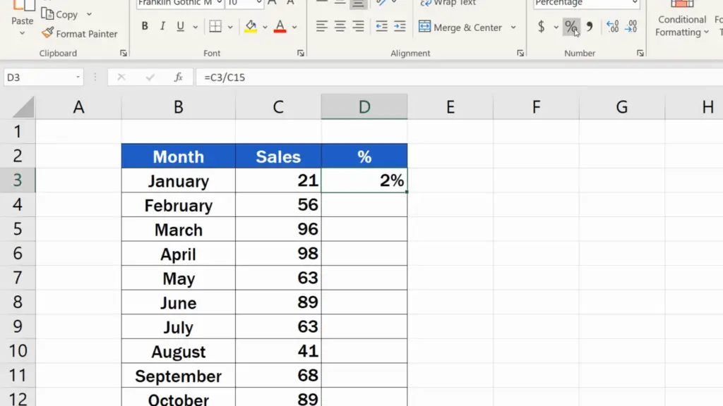
To make sure it displays correctly, we must properly format the cell with the formula. So, go to the Home tab, find ‘Number’ and click on the percent sign.

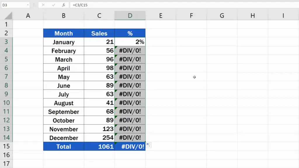
Now, if we try to copy the formula to the rest of the rows and calculate the percentage for the rest of the months, Excel shows an error. Why is that?

Relative Cell Reference

The thing is that Excel formulas standardly use so-called relative cell reference. This means that the formula in D3 uses the relative references to the cells C3 and C15, which is correct, but only in this row.

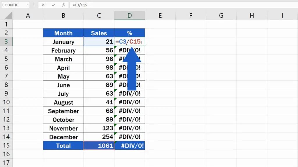
If we take a look at the formula copied one row below, we can see that the references have moved. The formula now contains the reference to C4, which is still fine, as we need to refer to the February value, but the second reference is C16, an empty cell and we need the formula to refer to the cell C15, which contains the value for total sales.

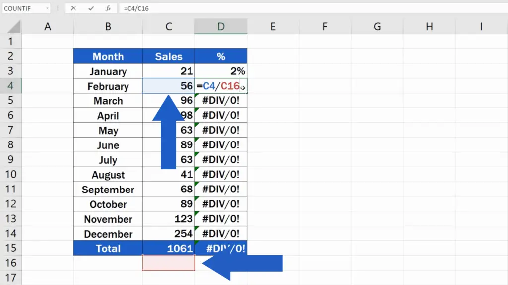
You can notice the same shift in each row.

So how to make the formula right, then? And here comes the moment to use the absolute cell reference.

How to Use Absolute Cell Reference Correctly

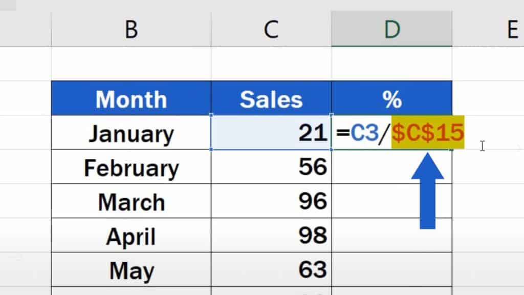
To make sure each row shows the correct value, we need to ‘lock’ the reference to the cell C15 in the first row, so that it wouldn’t change when copied to the rows below. Click into D3 and set the cursor on the reference C15. Press the Function key and then F4. Some of you might not need to use the Function key, this depends on the type of the keyboard you’re working with.

The reference to C15 has been marked with a dollar sign next to both the letter and the number, so we know that the reference has been ‘fixed’.

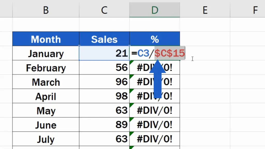
We have used the absolute reference to the cell C15, so that Excel would copy the formula that would divide the changing value in each row with the constant value from the cell C15.

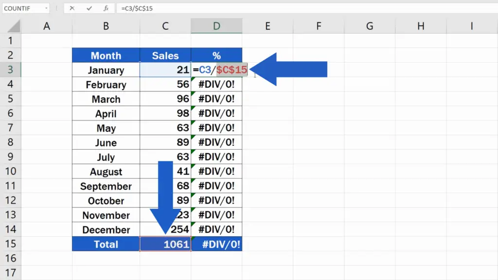
Once this is done, we press Enter and we can copy the formula to the rest of the rows safely.

Well done! The percentage now appears to be right!

When we click through all the rows containing the formula, we can see that Excel uses the same cell – C15 – everywhere.

For example, in row 4, the value from C4 is divided by C15 and in row 5, the value from C5 is divided by the value from the fixed cell reference C15, too.

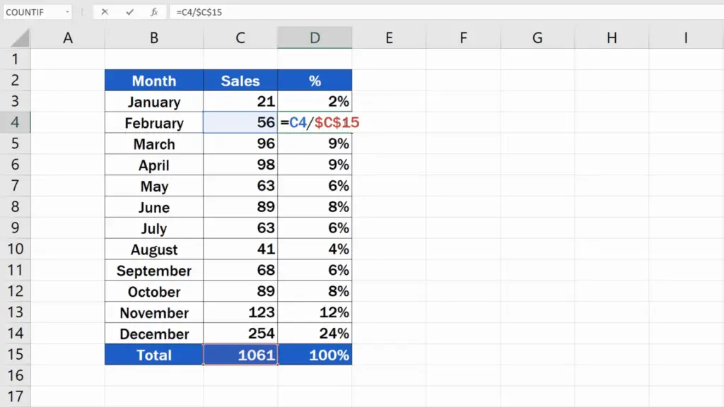
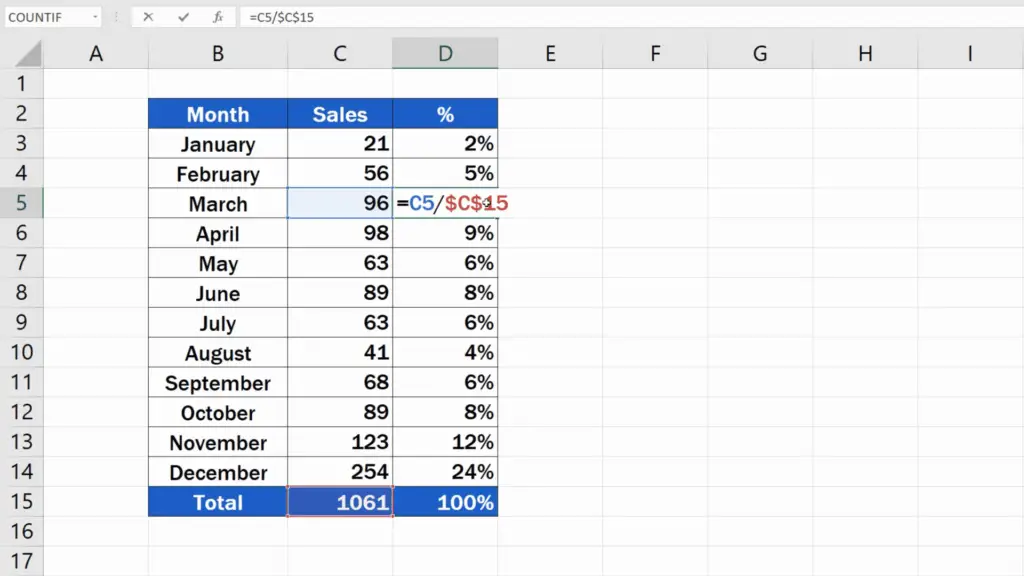
The calculations in all rows are correct. Thanks to the relative reference, the values for specific months are taken into account, but the absolute reference makes sure that the one and only value from the cell C15 for total sales is always used to work out the result correctly.

The absolute cell reference is effective whenever needed and works with any formula in Excel.

Don’t miss out a great opportunity to learn:

• How to Show Formulas in Excel
• How to Use the TODAY Function in Excel (Useful Examples Included)
• How to Use IF Function in Excel (Step by Step)
• How to Calculate the Range in Excel (in 3 easy steps)

If you found this tutorial helpful, give us a like and watch other video tutorials by EasyClick Academy. Learn how to use Excel in a quick and easy way!

Is this your first time on EasyClick? We’ll be more than happy to welcome you in our online community. Hit that Subscribe button and join the EasyClickers!

Thanks for watching and I’ll see you in the next tutorial!