How to Use SUMIF Function in Excel (Step by Step)

This tutorial offers a step-by-step guide on how to use the SUMIF function in Excel. This function works with a selected area, where it can quickly add values in the cells that meet specified criteria.

Let’s have a look at a couple of examples together!

Would you rather watch this tutorial? Click the play button below!

How the SUMIF Function Works

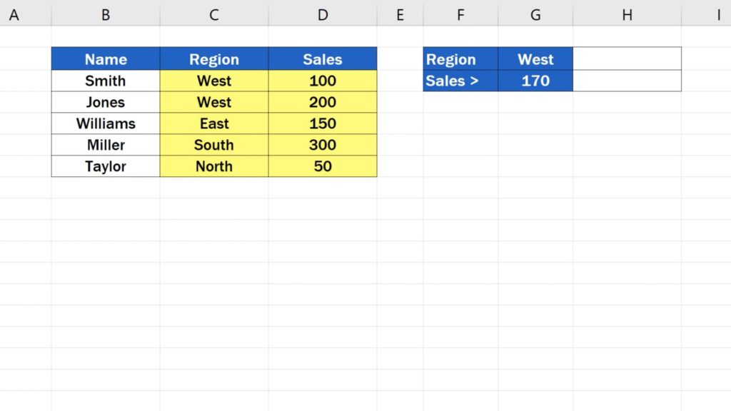
Here we’ve got some tables containing the data we’ll use to see how the SUMIF function works. For example, we can calculate the number of all sales made in the western region or find out the sum of all sales volumes that were below 170. And there’s no limit in terms of the amount of data in the tables!

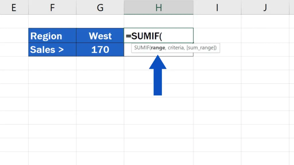
To begin, click into the cell you selected to display the result. Enter the equal sign and start typing ‘SUMIF’.

Click on the suggestion you’ll see and now you’ll need to enter some more information. Specifically, the range, which is the area of the cells where we need Excel to search for certain data; the criteria – to mark what exactly we’re looking for; and the area from which the sum of the values that meet our criteria will be calculated.

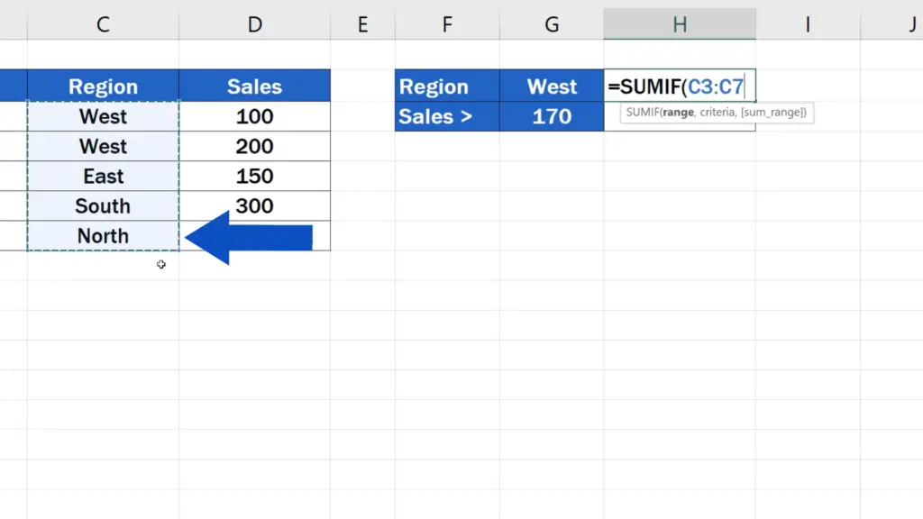
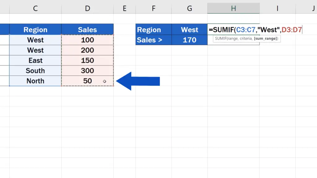
So, we want to search in the column Region, so we’ll select all the data in this column.

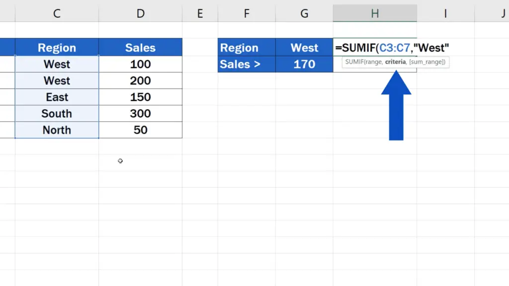
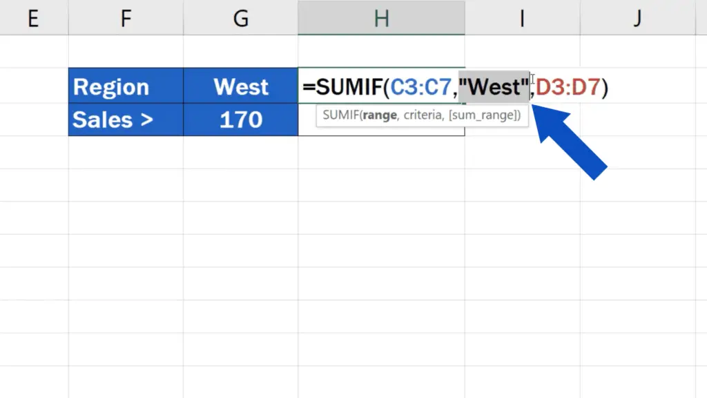
Then we’ll add a comma and enter the criteria. We want to find out the total of the sales from the region West, so we’ll type in “West” directly, in quotation marks.

Then a comma again, and now it’s time to select the area containing the values to be added, so select the column Sales.

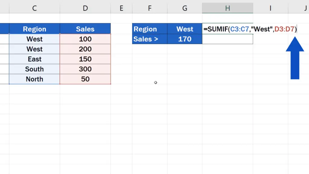
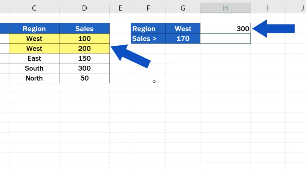
Close the brackets, hit Enter and here we go! Excel has calculated the total of all sales from the region West.

How to Use SUMIF function in Excel to Sum the Values in a Range that Meet Criteria

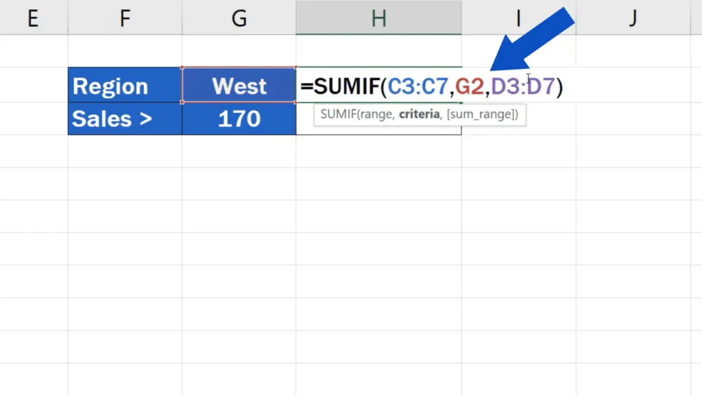
If you know that you’ll use different criteria to make different calculations in the future, you can adjust the function in a way that it will extract the necessary information from a single cell the contents of which you’ll be able to change anytime.

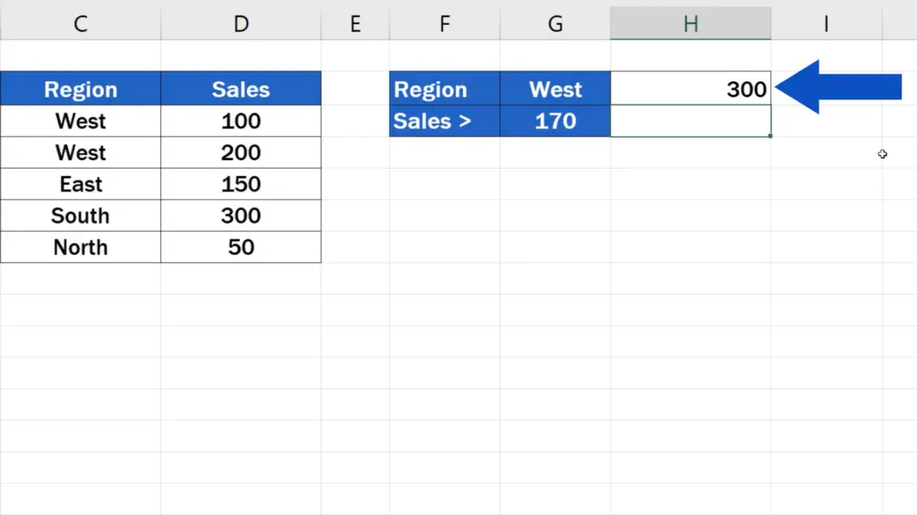
For example, to define our criteria, we want to use the value stated in the cell G2. So instead of typing the text “West” directly in the formula, we will use the coordinates G2 and press Enter. Great!

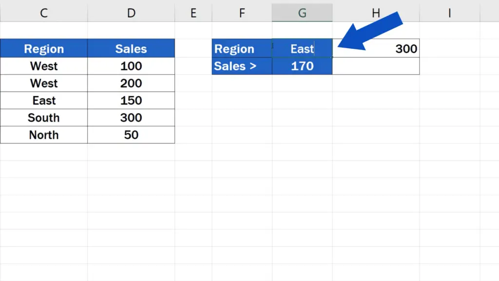
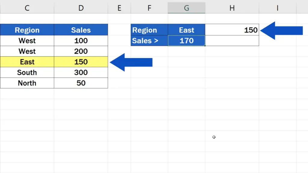
Now if we change West to East in G2, the formula recalculates the sum based on the most up-to-date criteria and we’ll see the total of all sales from the region East.

And that’s not all!

How to Use SUMIF function with Comparison Operator in Excel

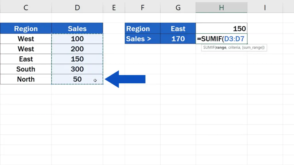
In the function SUMIF, you can also use comparison to find out the volume of all sales above or below the value you define. Let’s say we want Excel to add the volumes of sales larger than 170. We’ll start with the SUMIF function, select the column Sales.

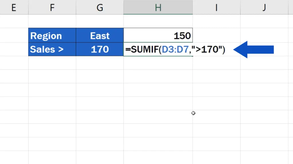
Add a comma and to write the comparison criteria directly, type in the symbol ‘greater than’ and the number 170, all in quotation marks. Now, in this kind of operation, Excel does not need any more information, so we’ll close the brackets and press Enter. And it works! Excel has provided us with the total of all sales entries greater than 170.

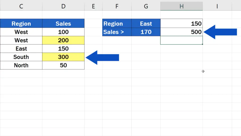
And it works! Excel has provided us with the total of all sales entries greater than 170.

As previously, in this case we can make the function dynamic, too. The cell G3 contains the data for the criteria information.

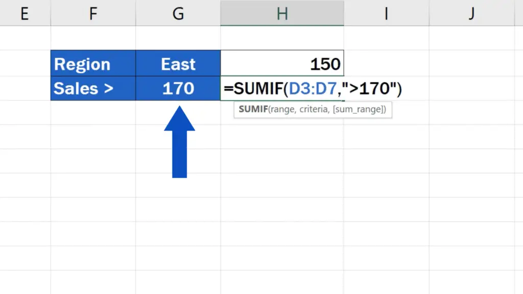
To use this number in the formula, we need to use a little trick, though. The sign ‘greater than’ needs to go into quotation marks, then we need to enter an ampersand and only then, we can type in the reference to the cell we want to use – G3.

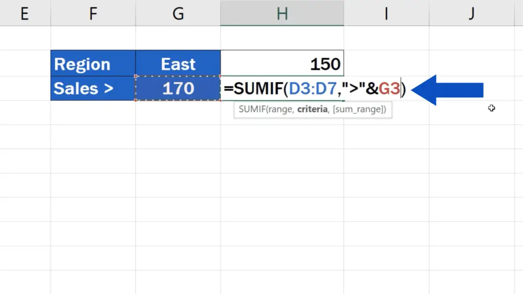
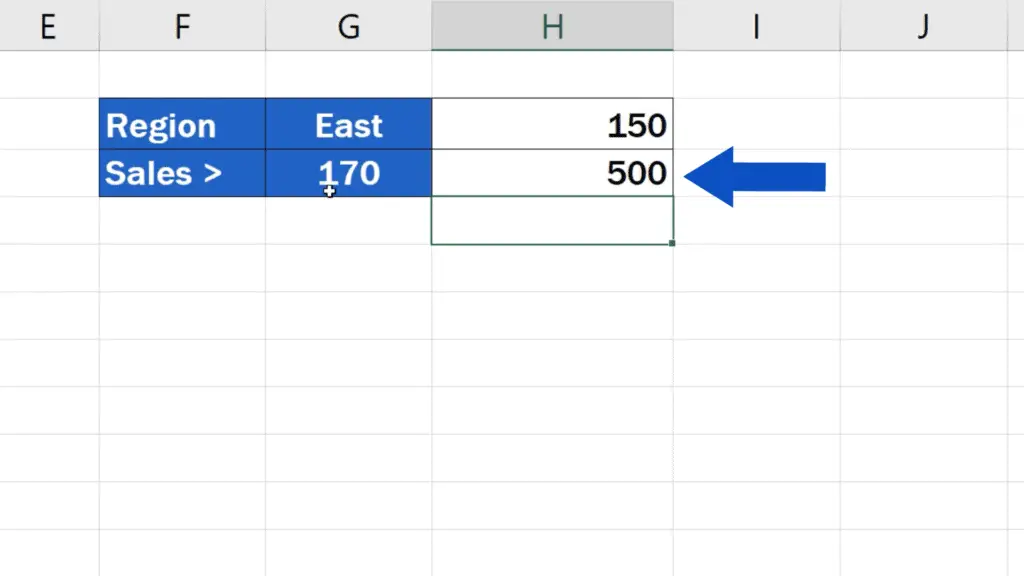
Now, we’ve got everything we needed, so we can press Enter and see that the spreadsheet shows the same result.

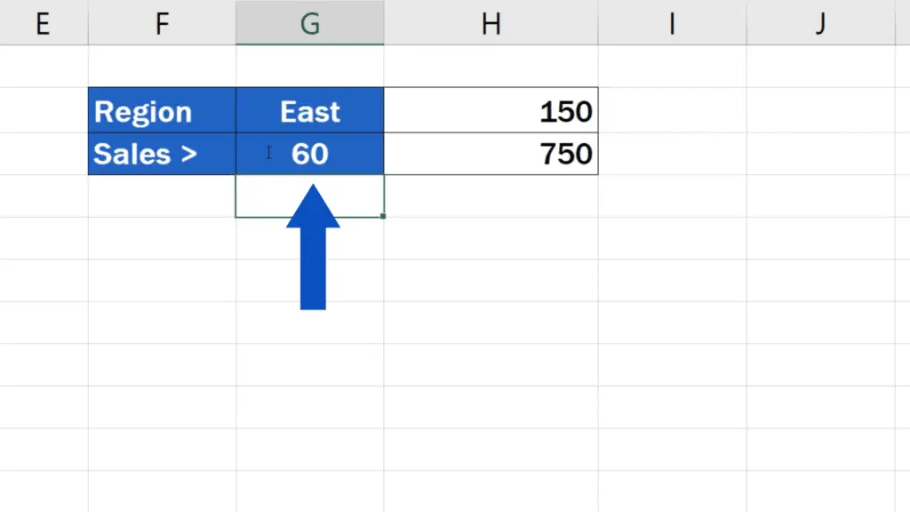
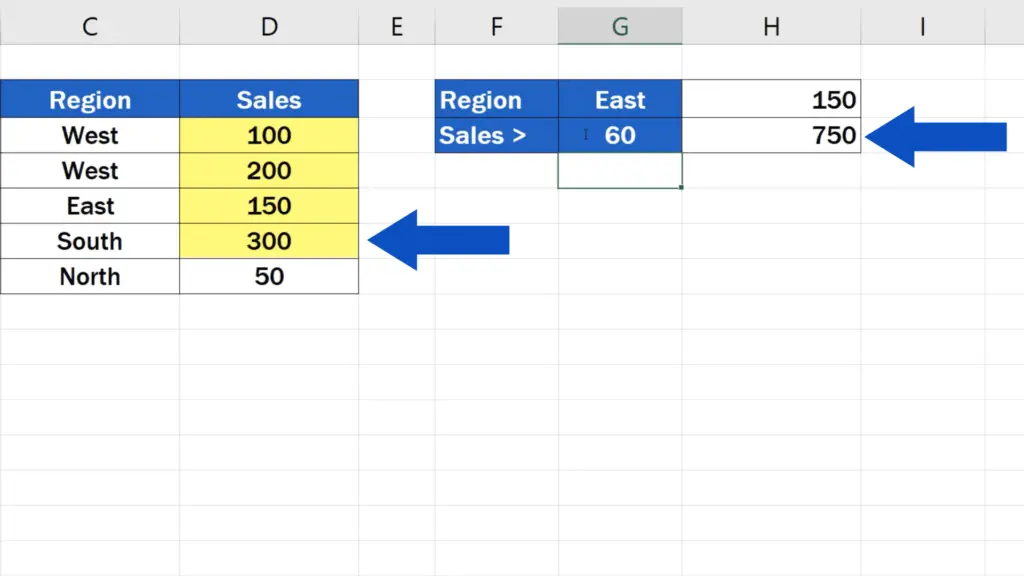
If we change the value in G3 to 60, Excel recalculates the total and shows the sum of all the sales that meet the new criteria, which is 750.

Well, that’s about all for today – we’ve seen how the function SUMIF works and how you can make use of it, for example at work.

But Excel offers a huge number of other helpful functions. EasyClick Academy has prepared the tutorials tutorials for the most popular ones – check out the links in the list below!

Don’t miss out a great opportunity to learn:

• How to Use the COUNTIF Function in Excel
• How to Use IF Function in Excel (Step by Step)
• How to Use Absolute Cell Reference in Excel
• How to Use the VLOOKUP Function in Excel (Step by Step)

If you found this tutorial helpful, give us a like and watch other video tutorials by EasyClick Academy. Learn how to use Excel in a quick and easy way!

Is this your first time on EasyClick? We’ll be more than happy to welcome you in our online community. Hit that Subscribe button and join the EasyClickers!

Thanks for watching and I’ll see you in the next tutorial!