How to Find a Circular Reference in Excel

Today’s video tutorial shows how to find a circular reference in Excel. A circular reference is an error which can completely block your calculations. Once you’ve watched this tutorial, you’ll be able to locate circular references in a spreadsheet and fix them in a quick and easy way.

What is a Circular Reference (Explained with Example)

A circular reference in Excel occurs when a formula refers to its own cell. In other words, the cell is trying to process a calculation using a formula that includes the cell itself, so basically, it uses the result before the calculation’s been done.

Let’s use this simple example to have a closer look at how it works.

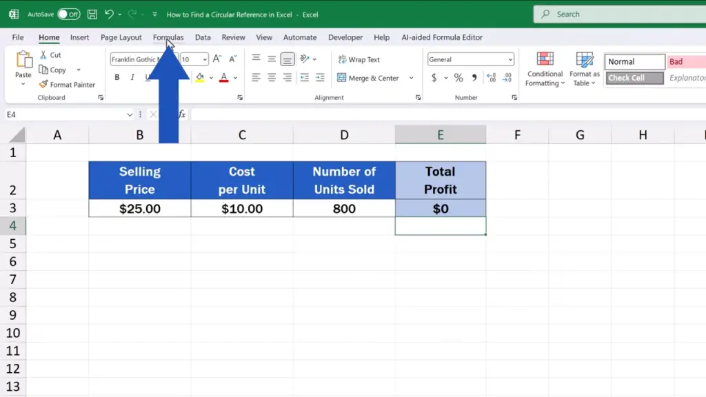
Column B contains ‘Selling Price’, column C includes ‘Cost per Unit’ and in column D, we can find ‘Number of Units Sold’. What we want to come up with is ‘Total Profit’ in column E.

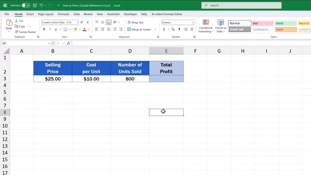
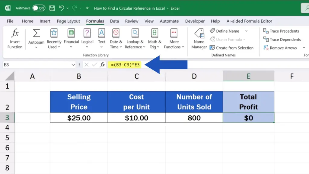
So, we write the formula for ‘Total Profit’ in the cell E3.

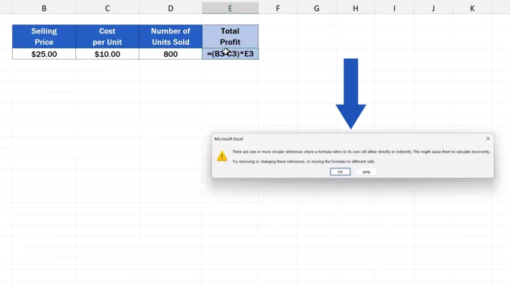
Here comes the equal sign, then we enter ‘B3’ minus ‘C3’ in parentheses followed by an asterisk and ‘E3’ to multiply the first part of the formula by the value in the cell E3.  

But watch out now! The formula contains an error – we’ve typed in the reference to the cell in which the formula is being written right now, which is E3.

Now, Excel is supposed to calculate a value from the cell E3 which has got no result yet. And that leads to an issue.

Immediately when the problem’s been detected, Excel shows this error message that states that the formula contains a circular reference. Of course, circular references usually happen with much more complicated calculations. Here, we’re using a very simple example for clarity.

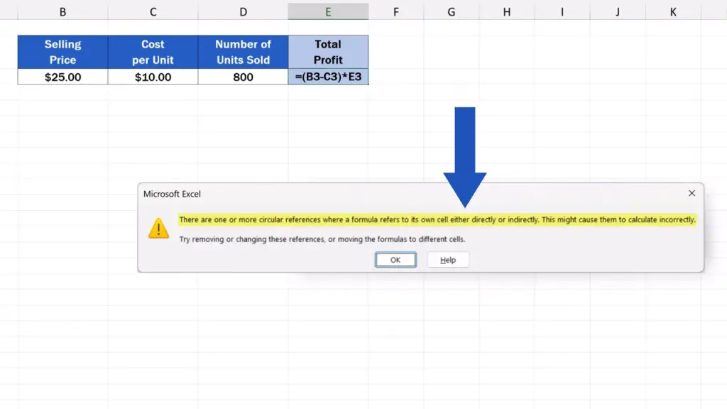
Once we see this message, we click on ‘OK’ and then we can have a look at a couple of ways to go through all the occurrences of circular reference in the spreadsheet so that we could fix them.

How to Detect Circular References in the Status Bar

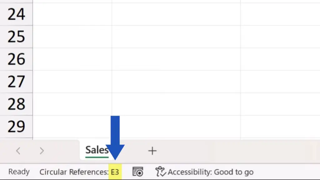
Another place where to check an occurrence of a circular reference in the spreadsheet is all the way down here, on the left, where we can also find various statuses and information.

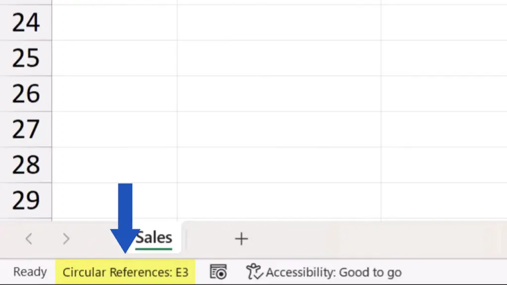
If you spot the notification ‘Circular References’, you’ll also see the exact cell where the issue’s occurred. In our case, E3 is the problem cell.

Before we fix this issue, we can check another important location where we can see that there’s a problem with circular references in the spreadsheet.

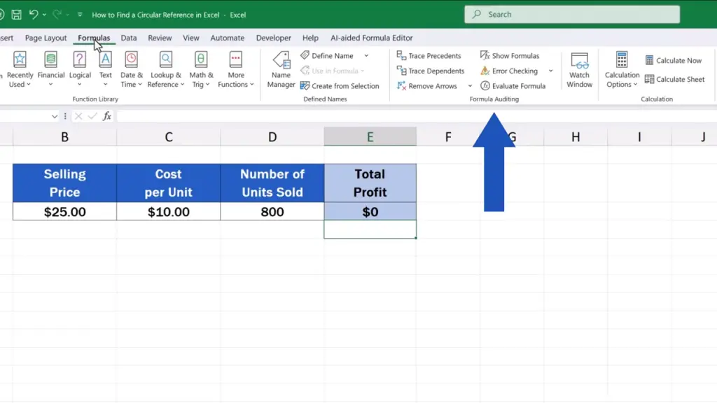
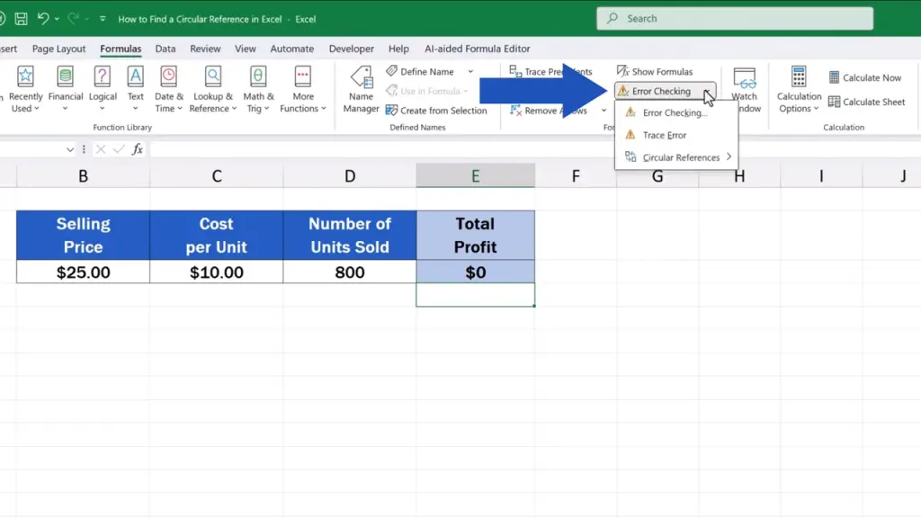
How to Find Circular References via the Formulas Tab

We navigate to the ‘Formulas’ tab, go to ‘Formula Auditing’, click on ‘Error Checking’ and all the way down here we find ‘Circular References’.

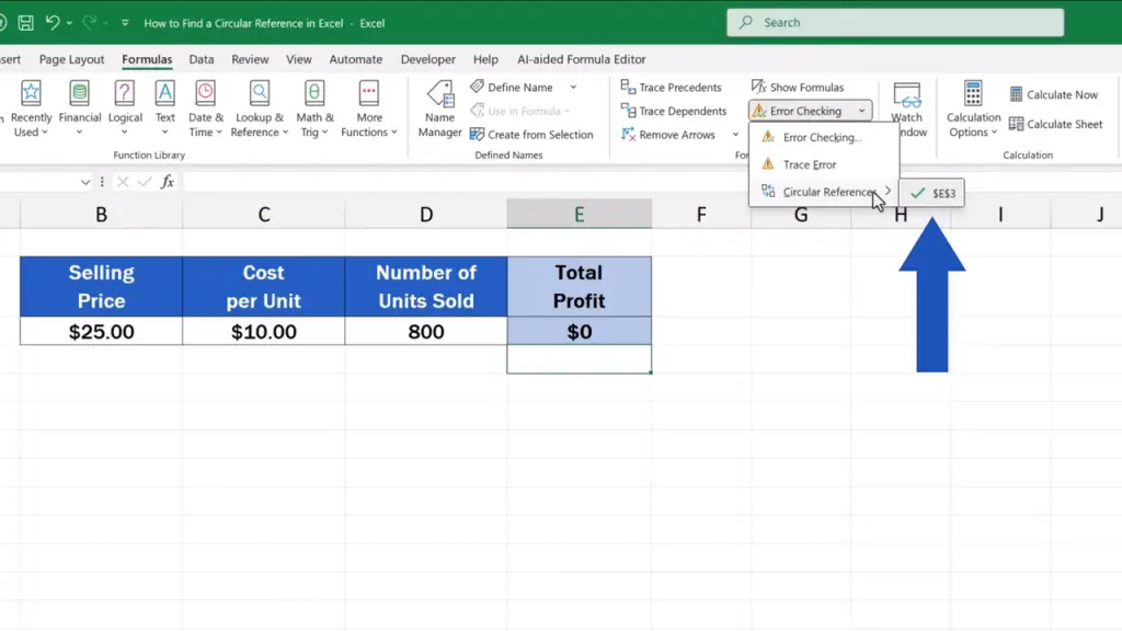
How to Fix a Circular Reference in Excelcell with issue

If there are more instances of circular reference, we’ll need to click on each one separately and fix each and every one of them.

If the list shows just one error, like we see right now, simply click on the entry and we’ll be redirected to the relevant cell.

And now, when we know where the problem is, we can try to fix it.

We check the entered formula thoroughly and, in our case it’s quite obvious, there’s an error in the ‘Total Profit’ formula – the reference to the cell E3 is wrong and we need to change that part to ‘D3’.

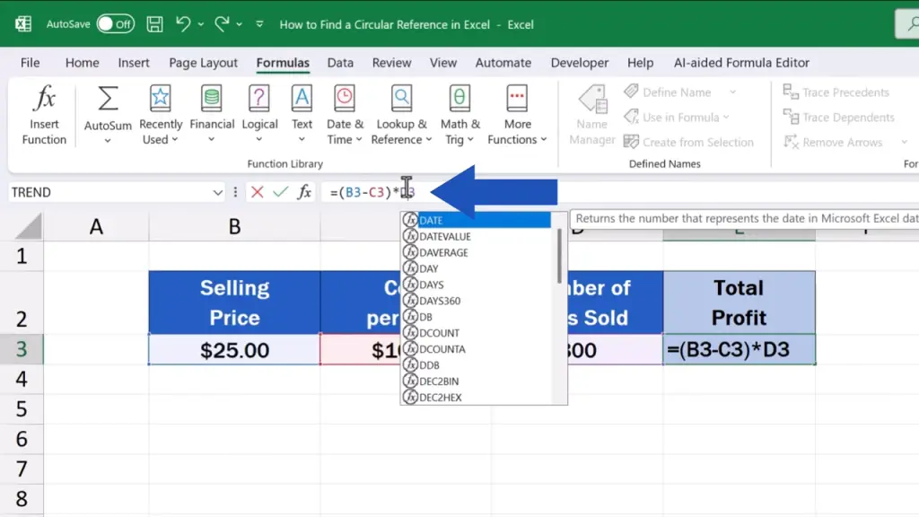
Now, we just hit Enter, and that’s all it takes! The error’s gone, the calculation’s working as it should!

Through this simple way, we can remove circular references in other, even more complicated calculations.

Don’t miss out a great opportunity to learn:

• How to Remove Blank Rows in Excel – BASIC
• How to Remove Blank Rows in Excel – ADVANCED
• How to Change Date Format in Excel (the Simplest Way)

If you found this tutorial helpful, give us a like and watch other tutorials by EasyClick Academy. Learn how to use Excel in a quick and easy way!

Is this your first time on EasyClick? We’ll be more than happy to welcome you in our online community. Hit that Subscribe button and join the EasyClickers!

Thanks for watching and I’ll see you in the next tutorial!